Testing the validity of the neoclassical migration model: Overall and age group specific estimation results for German spatial planning regions

Munich Personal RePEc Archive

Testing the validity of the neoclassical

migration model: Overall and age-group

specific estimation results for German

spatial planning regions

Mitze, Timo and Reinkowski, Janina

RWI Essen

12 July 2010

Online at

https://mpra.ub.uni-muenchen.de/23835/

Testing the Validity of the Neoclassical Migration

Model: Overall and Age-Group Specific Estimation

Results for German Spatial Planning Regions

Timo Mitze∗ _{Janina Reinkowski}∗∗

This Version: July 2010

Abstract

This paper tests the empirical validity of the neoclassical migration model in predicting German internal migration flows. We estimate static and dynamic migration functions for 97 Spatial Planning Regions between 1996–2006 using key labour market signals including income and unemployment differences among a broader set of explanatory variables. Beside an aggregate specification we also estimate the model for age-group related subsamples. Our results give empirical support for the main transmission channels identified by the neoclassical framework: That is, regional differences in the real income show the expected positive effect on the net inmigration rate, while the link between regional unemployment rate differentials and net inmigration is negative. The results remains stable if further variables are added to the model. Net in-commuting shows a negative correlation with in-migration underlying the substitutive nature of the two variables. Moreover an increasing level of international competitiveness attracts further in-migration flows. We also find heterogeneity for different types of settlement structure and the East-West macro regions by including federal state level fixed effects or an East German dummy. The results broadly hold for age-group specific estimates. Here, the impact of labour market signals is tested to be of greatest magnitude for workforce relevant age-groups and especially young cohorts from 18 to 25 and 25 to 30 years. This latter result underlines the prominent role played by labour market conditions in determining internal migration rates of the working population in Germany.

JEL: R23, C31, C33

Keywords: German Internal Migration, Harris-Todaro Model, Dynamic Panel Data

∗_{Corresponding Author. RWI Essen. – All correspondence to: Timo Mitze, RWI, Hohenzollernstr. 1-3, 45128 Essen,} Germany, e-mail: [email protected]. Tel.: +49(0)201/8149–223, Fax: +49(0)201/8149–200.

Zur Validit¨

at des Neoklassischen Migrationsmodells:

Aggregierte und Altersgruppen-Spezifische Sch¨

atzergebnisse

f¨

ur Deutsche Raumordnungsregionen

Zusammenfassung

1

Introduction

There are many theories aiming to explain, why certain people migrate and others do not. However, the neoclassical model remains still the standard workhorse specification to analyse internal and external migration rates at the regional, national and international level. The model puts special emphasis on the labour market dimension of migration and basically relates migration-induced population changes as a response to relative income (or wage) and employment situations found in the origin and destination region. Migration then itself works as an equilibrating mechanism for balancing differences among regions with respect to key labour market variables since higher in-migration in a region is ex-pected to reduce the regional wage level due to an increase in labour supply. From the perspective of economic policy making the empirical implications of the neoclassical mi-gration model are important to assess whether labour mobility can act as an appropriate adjustment mechanism in integrated labour markets facing asymmetric shocks. Though the neoclassical migration model is widely used as a theoretical and didactic tool, the international empirical evidence provides rather mixed results.

In this paper, we therefore aim to check the validity of the neoclassical migration model using a panel of 97 German regions for the period 1996 – 2006. We are especially interested in taking a closer look at the role played by dynamic adjustment processes driving the internal migration patterns. We also aim toto identify likely role played by additional factors as well as regional amenities in explaining migratory movements beside key labour market signals and focus on the heterogeneity of adjustment processes taking place when migration flows are disaggregated by age groups.

2

The neoclassical migration model

Theories of migration try to explain what drives population flows. Given the complex nature of the decision process individuals face, there is a large variety of theoretical models available to explain the actual migration outcome. These models may either be classified as micro- or macroeconomic in nature. While micro behavioural models focus on dominant factors at the individual level (such as the human capital model as outlined for example in Sjaastad, 1962), macroeconomic models especially focus on the labour market dimension of migratory flows.

Given the strong need for a solid microeconomic foundation of many macro relati-onships, the neoclassical migration framework also starts from a micro-founded lifetime expected income (utility) maximization approach as specified in the classical work done on the human capital model of migration. The latter model in fact views the process of migration as an investment where the returns to migration in terms of higher wages asso-ciated with a new job exceed the costs involved in moving. Relaxing the assumption that the potential migrant has perfect information about the wage rates and job availabilities among all potential locations involved in his decision making process, Todaro (1969) was among the first to propose a model where the potential migrant discounts wages by the probability of finding a job in respective regions. From this follows that throughout the decision making process, the individual compares the expected (rather than known) inco-me he would obtain for the case he stays in his hoinco-me region (i) with the expected income we would obtain in the alternative region (j) and further accounts for ’transportation costs’ of moving from region i toj.

In their seminal paper, Harris & Todaro (1970) further formalize this idea: The authors set up a model where the expected income from staying in the region of residence YE

ii is a

function of the wage rate or income in regioni(Yi) and the probability of being employed

(P rob(EM Pi)). The latter in turn is assumed to be a function of unemployment rate in

region i (Ui) and a set of potential variables related both to economic and non-economic

factors (Xi). The same set of variables - with different subscripts for regionj accordingly

- is also used to model the expected income from moving to an alternative region. Thus, taking costs of moving from region itoj into account (Cij), the individual’s decision will

be made in favour of moving to region j if

YiiE < Y E

ij −Cij, (1)

where YE

ii = f(P rob(EM Pi), Yi) and YijE = f(P rob(EM Pj), Yj). The potential

probability of finding employment. Using this information, we can set up a model for the regional net migration rate (N Mij) defined as regional in-migration flows to i fromj

relative to outmigration flows fromitoj (possibly normalized by the regional population level), which has the following general form:

IN Mij −OU T Mij =N Mij =f(Yi, Yj, Ui, Uj, Xi, Xj, Cij). (2)

With respect to the theoretically motivated signs of the explanatory variables we expect that an increase in the home country wage rate (or, alternatively, the real income level)

ceteris paribus leads to higher net migration inflows, while a wage rate increase in region

j results in a decrease of the net migration rate. On the contrary, an increase in the unemployment rate in region i (j) has negative (positive) effects on the bilateral net migration from i to j. The costs of moving from i to j are typically expected to be an impediment to migration and thus are negatively correlated with net migration as:1

∂N Mij ∂Yi

>0;∂N Mij

∂Yj

<0;∂N Mij

∂Ui

>0;∂N Mij

∂U j <0;

∂N Mij ∂Cij

<0. (3)

Core labour market variables may nevertheless not be sufficient to predict regional migration flows. Recent extensions of the model therefore include further driving forces of migration such as human capital, the regional competitiveness, housing prices, population density and environmental conditions, among others (see e.g. Napolitano & Bonasia, 2010, for an overview). We refer to the neoclassical migration model focusing solely on labour market conditions as the ’baseline’ specification, while the ’augmented’ specification also controls for regional amenities and further driving forces such as population density and commuting flows as a substitute for migratory movements.

Moreover, regional amenities are typically included as a proxy variable for (unobserved) specific climatic, ecological or social conditions in a certain region. According to the amenity approach regional differences in labour market signals then only exhibit an effect on migration after a critical threshold has been passed. Since in empirical terms it is often hard to operationalize amenity relevant factors, Greenwood et al. (1991) propose to test the latter effect by the inclusion (macro-)regional dummy variables in the empirical model. For the long run net migration equation amenity-rich regions then should have dummy coefficients greater than zero (and vice versa), indicating that those regions exhibit higher than average in–migration rates as we would expected after controlling for regional labour market and macroeconomic differences.

1_{The migration effect of the vector of further economic variablesX}

The baseline and augmented migration equations can then either be applied at the micro-, regional or macroeconomic level. The advantage of studies at the macro level is that an analysis of the elasticity of migration with respect to income and unemployment changes gives important information about the size of the adjustment process taking place of balance cross-regional labour market difference through labour migration. In the next section, we therefore estimate the short and long-run impact of alterations in unemployment rates and incomes on migration. Using a flexible estimation approach we also seek to determine whether economic disparities appear to be necessary but not sufficient condition for observed migration processes. The latter hypothesis would give rise to a significant role played by other factors such as local amenities besides labour market signals.

The likely impact of these latter variables in the augmented neoclassical framework can be sketched as follows: Taking human capital as an example, it may be quite reasonable to relax the assumption of the Harris-Todaro model that uneducated labour has the same chance of getting a job as educated labour. Instead, the probability of finding a job is also a function of the (individual but also region specific) endowment with human capital (HK). The same logic accounts for regional competitiveness (IN T COM P): Here, we expect that those regions with a high competitiveness are better equipped to provide job opportunities than regions lagging behind (where regional competitiveness may e.g. be proxied by the share of foreign turnover relative to total turnover in sectors with internationally tradeable goods). For population density (P OP DEN S), we expect in general a positive impact of agglomeration forces on net flows through an increased possibility of finding a job, given the relevance of spillover effects e.g. from a large pooled labour market. Thus the probability of finding employment in region i in the augmented neoclassical migration model takes the following form:2

P rob(EM Pi) = f[Ui, HKi, IN T COM Pi, P OP DEN Si], (4)

with: ∂N Mij

∂HKi

>0; ∂N Mij

∂IN T COM Pi

>0; ∂N Mij

∂P OP DEN Si >0.

Finally, we also carefully account for alternative adjustment mechanisms to restore the inter-regional labour market equilibrium such as net commuting flows as substitute to migratory movelents. Here we expect that these flows are negatively correlated with net inmigration.

2_{The opposite effect onN M}

3

Econometric Specification

For the empirical estimation of the neoclassical migration model we start from a core specification as e.g. applied in Puhani (2001) and set up a model for the net migration rate as:

N Mij,t P OPi,t−1

!

=Ai,t

Ui,tα1−1Yi,tα2−1 Uα3

j,t−1Y α4 j,t−1

!

, (5)

where net migration rate between i and j is defined as regional net balance N M for regionirelative to the rest of the countryj,P OP is the region’sipopulation level,tis the time dimension.3 _{A is a (cross-section specific) constant term. In the empirical literature}

a log-linear stochastic form of the migration model in eq.(5) is typically chosen as (where lower case variables denote logs) and nmrij,t=log(N Mij,t/P OPi,t−1):

nmrij,t = α0+α1yi,t−1+α2yj,t−1 (6)

+α3ui,t−1+α4uj,t−1+α5X+eij,t,

where the error termeij,t=µij+νij,thas the typical error component structure. Taking

into account that migration flows typically show some time persistence, we augment eq.(6) by the lagged value of net migration as:

nmrij,t = β0+β1nmrij,t−1+β2yi,t−1+β3yj,t−1 (7)

+β4ui,t−1+β5uj,t−1+β6X+uij,t,

The inclusion of a lagged dependent variable can be motivated by the existence of social networks in determining internal migration flows over time: That is, Rainer & Siedler (2009) for example find for German micro data that the presence of family and friends is indeed an important predictor for migration flows in terms of communication links, which may result in a time dependence of the adjustment path for migration flows out of particular origin to destination regions. Finally, in applied work one typically finds a restricted version of eq.(7) where net migration is regressed against regional differences of explanatory variables of the form (see e.g. Puhani, 2001)

nmrij,t=γ0+γ1nmrij,t−1+γ2y˜ij,t−1+γ3u˜ij,t−1+γ4X+uij,t, (8)

where ˜xij,t for a variable xij,t denotes ˜xij,t=xi,t−xj,t. The latter specification implies

the following testable restrictions of the unrestricted model in eq.(8), for which we will account for in the empirical estimation:

β2 = −β3, (9)

β4 = −β5. (10)

For estimation purposes we then have to find an appropriate estimator, which accounts for the above described empirical setup. Given the dynamic nature of the neoclassical migration model in eq.(8) we can write the specified form in terms of a more general dynamic panel data model as (in log-linear specification):

yi,t =α0+α1yi,t−1+ k

X

j=0 β′

jXi,t−j +ui,t, with: ui,t =µi+νi,t, (11)

again i = 1, . . . , N (cross-sectional dimension) and t = 1, . . . , T (time dimension).

yi,t is the endogenous variable and yi,t−1 is one period lagged value. Xi is the vector of

explanatory time-varying and time invariant regressors, ui,t is the combined error term,

where ui,t is composed of the two error components µi as the unobservable individual

effects and νi,t is the remainder error term. Both µi and νi,t are assumed to be i.i.d.

residuals with standard normality assumptions.

There are numerous contributions in the recent literature with respect to the single equation estimation of the dynamic model of the above type, which especially deal with the problem introduced by the inclusion of a lagged dependent variable in the estimation equation and its built-in correlation with the individual effect: That is, since yit is also

a function of µi, yi,t−1 is a function of µi and thus yi,t−1 as right-hand side regressor in

eq.(11) is correlated with the error term. Even in the absence of serial correlation ofνitthis

renders standard OLS, FEM and REM models biased and inconsistent (see e.g. Nickel, 1981, Sevestre & Trogon, 1995 or Baltagi, 2008, for an overview).

System GMM estimator by Blundell & Bond (1998), which builds consistent instruments based on the following orthogonality conditions:

E(yi,t−ρ∆ui,t) = 0 for all ρ= 2, . . . , t−1, (12)

where ∆ is the difference operator defined as ∆ui,t =ui,t−ui,t−1. Eq.(12) is also called

the ’standard moment condition’ and is widely used in empirical estimation. However, one general drawback of dynamic model estimators in first differences is their poor empirical performance especially for a high persistence in the autoregressive component such as growth models (see Munnel, 1992, and Holtz-Eakin, 1994, for poor empirical estimates of a production function in FD, Bond et al. (2001) for growth equation estimates). Bond et al. (2001) argue that first difference IV/GMM estimators can be poorly behaved, since lagged levels of the time series provide only ’weak instruments’ for sub-sequent first-differences.

E(∆yi,t−1ui,t) = 0 for t=3,...,T. (13)

Rather than using lagged levels of variables as instruments for the equation in first difference according to eq.(12), eq.(13) defines an orthogonality condition for the model in level that uses instruments in first differences. Blundell & Bond (1998) propose the system GMM estimator as combination of both orthogonality conditions.

In our estimation design we are especially interested in testing for the appropriateness of the chosen IV approach and apply test routines that account for the problem of many and/or weak instruments in the regression (see e.g. Roodman, 2006). Moreover, as it is typically the case with regional data we are especially aware of the potential bias induced by a significant cross-sectional dependence in the error term of the model. There are different ways to account for such error cross-sectional dependences implying

Cov(νi,tνj,t)6= 0 for some t and i6=j (14)

(see e.g. Sarafidis & Wansbeek, 2010, for an overview). Besides the familiar spatial ap-proach, recently the common factor structure approach has gained considerable attention. The latter specification assumes that the disturbance term contains a finite number of unobserved factors that influence each individual cross-section separately. In terms of the above described combined residual term of the dynamic panel data model in eq.(11), we are able to introduce a common factor structure for the error term in the following way:

ui,t =µi+νi,t, νi,t = M

X

m=1

φm,ifm,t+ǫi,t, (15)

unobserved effects, φi = (φ1,i, . . . , φM,i)′ is an M × 1 vector of factor loadings and ǫi,t

is a pure idiosyncratic error component with zero mean and constant variance. Cross-sectional dependence in turn leads to inconsistent estimates if regressors are correlated with the unspecified common variables or shocks. There are different proposals in the li-terature to account for unobserved factors. For dynamic panel estimators with short time dimension, Sarafidis & Robertson (2009) propose to apply time-specific demeaning which alleviates the problem of parameter bias if the variance of the individual factor loadings for the common factor models is small. Alternatively, if the impact of the common fac-tor varies considerably by cross-sections, there are different estimation techniques, which account for cross-sectional dependence by using cross-section averages of the dependent and independent variables as additional regressors (see e.g. Pesaran, 2006).

Recently, various testing procedures have been developed to check for the presence of cross-sectional dependence. Among the most commonly applied routines is Pesaran’s (2007) extension to the standard Breusch & Pagan LM test. The so-called Cross-Section Dependence (CD) test is based on the pairwise correlation coefficient of residuals from a model specification that ignores the potential presence of cross-sectional dependence. However, as Sarafidis & Wansbeek (2010) point out, the CD-Test has the weakness that it may lack power to detect the alternative hypothesis under which the sign of the elements of the error covariance matrix is alternating (thus for positive and negative correlation in the residuals, e.g. for factor models with zero mean factor loadings). Moreover, the test statistic requires normality of the residuals. Thus, Sarafidis et al. (2009) propose an alternative testing procedure that does not require normality and is valid for fixed T and large N. The testing approach designed for the Arellano-Bond (1991) and Blundell-Bond (1998) GMM estimators is based on Sargan’s difference-test statistic for overidentifying restrictions. The aim of the test is to examine whether there is still (heterogeneous) cross-sectional dependence in the residuals after time-specific demeaning in the logic of Sarafidis & Robertson (2009). The test has the following simple (C-Statistic based) form:4

CCD−GM M = (SF −SR) d

→χ2_hd, (16)

where hd is the number of degrees of freedom of the test statistic as difference

bet-ween the set of instruments (number of moment conditions) in the full model (SF) and

the restricted model (SR), where the GMM model has either the Arellano-Bond or the

Blundell-Bond form augmented by time-specific dummy variables. The corresponding null

hypothesis of the Sargan’s difference-test tests is that there is homogeneous cross-section dependence in the model versus the alternative of heterogeneous cross-section dependence as:5

H0 : Var(φi) =

X

φ= 0 versus: H1 :X

φ6= 0. (17)

The restricted (sub-)set of moment conditions thereby only includes instruments from regressors in the vector Xi,t (according to eq.(11)) that remain strongly exogenous in the

sense that their factor loadings are mutually uncorrelated with the cross-section specific parameter of the the common factor. Sarafidis et al. (2009) propose to likewise test for the exogeneity of a subset of regressors by means of the standard Sargan’s/Hansen’s test for overidentifying restrictions in a first step.6

Before estimating the model and testing for the appropriateness of alternative specifi-cation we first discuss recent findings in the empirical literature and present some stylized facts of German internal migration and regional economic and social characteristics. We also check for the time-series properties of the variables involved in order to avoid any spurious regression problem associated with non-stationary data.

4

What does the empirical literature say?

Testing for the empirical validity of the (baseline) neoclassical migration model for inter-nal migration in European countries yields rather mixed results:7 _{Regional disparities in}

(un-)employment are often shown to be important factors in determining migratory flows. On the contrary, the influence of regional wage or income levels is difficult to prove in many empirical examinations (see e.g. Pissarides & McMaster, 1990, as well as Jackman and Savouri (1992) for British regions; Westerlund, 1997, for inter-regional migration in Sweden, Devillanova & Garcia-Fontes, 2004, for Spain). Only for the Italian case Daveri & Faini (1998) show that the regional wage level corresponds to the theoretically expec-ted signal for the gross outward migration from southern to northern regions. Similar results are found in Fachin (2007). Napolitano & Bonasia (2010) show that although the coefficients for Italian labour market variables in the neoclassical migration model shows the expected sign, due to the complexity of the internal migration process, the baseline Harris-Todaro approach neglects important variables such as agglomeration forces

measu-5_{If only homogeneous cross-section dependence is present the inclusion of time-specific dummies variables is sufficient to} remove any bias in the estimation approach, see e.g. Sarafidis & Robertson (2009).

6_{One has to note that instruments derived from transformations the lagged endogenous regressor cannot be included in} the subset of strictly exogenous moment conditions to test for the null hypothesis of homogeneous cross-section dependence.

red by population density and human capital. The latter variable is also found significant besides the standard labour market variables in an inter-regional migration model for the Polish transition process (see Ghatak et al., 2008).

For German interregional migration, Decressin (1994) examined gross migration flows for West German states up to 1988. His results show that a wage increase in one region relative to others causes a disproportional rise in the gross migration levels in the first region, while a rise in the unemployment in a region relative to others disproportionally lowers the gross migration levels. Decressin does not find a significant connection between bilateral gross migration and regional differences in wage level or unemployment when purely cross-sectional estimate are considered. Difficulties in proving a significant influence of regional wage decreases on the migratory behavior within Germany are also found in earlier empirical studies based on micro-data directly addressing the motivation for individual migratory behavior in Germany. Among these are Hatzius (1994) for the West German states, and Schwarze and Wagner (1992), Wagner (1992), Burda (1993) and Buechel & Schwarze (1994) for East Germany. Subsequent studies succeed in qualifying the theoretically unsatisfactory result of an insignificant wage influence: Schwarze (1996) shows that by using the expected wage variables instead of the actual ones, the wage drop between East German and West German states has a significant influence on the migratory behavior.8 _{In a continuation of Burda (1993), Burda et al. (1998) also indicates}

a significant non-linear influence on household income.

Contrary to earlier evidence, in recent macroeconomic studies with an explicit focus on intra-German East-West migration flows, regional wage rate differentials are broadly tested to significantly affect migration flows (see e.g. Parikh & Van Leuvensteijn, 2003, Hunt, 2000, as well as Burda & Hunt, 2001). The study of Parikh & Van Leuvensteijn (2003) augments the core migration model with regional wage and unemployment diffe-rentials as driving forces of interregional migration by various indicators such as regional housing costs, geographical distance and inequality measures. For the sample period 1993 to 1995, the authors find a significant non-linear relationship between disaggregated re-gional wage rate differences and East-West migration (of a U-shaped form for white-collar workers and of inverted U-form for blue-collar workers), while unemployment differences are tested be insignificant. The relationship between income inequality and migration did not turn out to be strong.

According to Hunt (2000) and Hunt & Burda (2001), wage rate differentials and

ally the fast East-West convergence are also a significant indicator in explaining observed state-to-state migration patterns. Using data from 1991 to 1999, Hunt & Burda (2001) find that the decline in East-West migration starting from 1992 onwards can almost exclu-sively be explained by wage differentials and the fast East-West wage convergence, while unemployment differences do not seem to play an important part in explaining actual migration trends.9 _{In a recent application, Alecke et al. (2010) apply Panel VAR}

techni-ques to analyse the simultaneous impact of labour market variables to migration and vice versa for German Federal States between 1991 and 2006. The results broadly support the neoclassical migration model and show that migration itself has an equilibrating effect on labour market differences. The authors also find evidence for structural differences between the West and East German macro regions in the migration equation, similar to findings for an Italian ’empirical puzzle’ with a distinct North-South division in terms of the magnitude of the migration response with respect to labour market signals (see e.g. Fachin, 2007, and Etzo, 2007).

5

Data and stylized facts of German internal migration

Given the heterogeneity found in the international empirical literature in predicting inter-regional migration flows, we take these results as a starting point for an updated regression approach based on German spatial planning units between 1996 and 2006. For empirical estimation we use regional data for the 97 German Spatial Planning Regions (so called

Raumordnungsregionen) as the level of analysis for spatial migration processes within Germany (see e.g. Bundesinstitut fuer Bau-, Stadt-, und Raumforschung, 2010, for details about the concept of Spatial Planning Regions). The time period used for estimation ranges from 1996 to 2006. We have chosen to restrict our estimation approach to this period since the regional boundaries of the German Spatial Planning Regions have changed before and after, which may introduce a measurement problem that is likely to bias our empirical results.

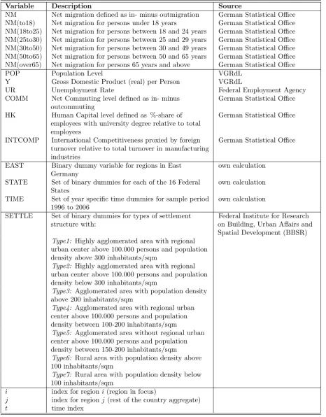
We use variables for regional net migration, population, real income, the unemployment rate, human capital endowment, international competitiveness of regions and commuting flows. The latter has been included to account for an alternative adjustment mechanism to balance labour market disequilibria. We also include two sets of dummy variables in-to the migration model: 1.) binary dummy variables for the 16 federal states in-to capture macro regional differences. This may be especially important to account for structural

differences between West and East Germany (see e.g. Alecke et al., 2010, for recent fin-dings); 2.) binary dummy variables for different regional settlement types ranging from metropolitan agglomerations to rural areas (in total 7 different categories based on their absolute population size and population density). As Napolitano & Bonasia (2010), point out variables measuring population density may be an important factor in explaining the regional amenities. Variable definitions and descriptive statistics are provided in table 1 to 3.

<<< Table 1 to table 3 about here >>>

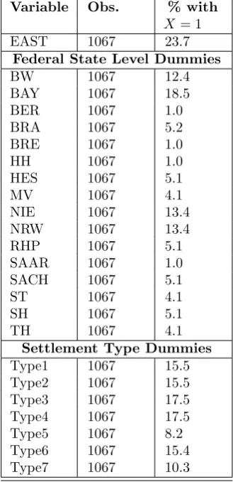
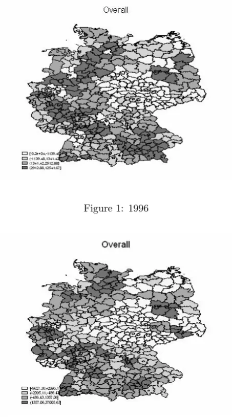
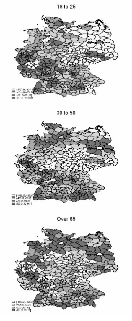
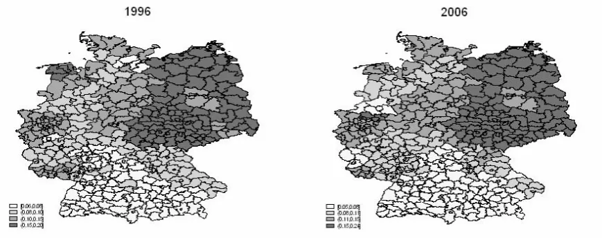
In order to show some distinct regional and macro-regional differences for net migrati-on and explanatory variables, figure 1 to figure 6 additimigrati-onally visualize the above shown descriptive statistics for net migration and labour market variables. As figure 1 shows for both periods 1996 and 2006, the net in-migration flows show a high level of persis-tence with huge net losses for the northern south-western regions in East Germany. Also, the Western regions along the border to East Germany experienced net outflows. On the other hand the northern West German Spatial Planning Regions around the urban agglomerations Hamburg and Bremen are among the net inflow regions as well as the western agglomerated regions in the Rhineland (around the metropolitan areas Cologne and Duesseldorf) and the southern West German regions in Baden Wuerttemberg and Bavaria. Among the few regions in East Germany with net migration inflows is the belt of regions around Berlin. Looking at net migration trends by age-groups in figure 2 and 3 the graphs show that especially net outflows of the East German regions are especially prevailing for the age-group of young persons between 18 and 25 years. This may give a first indication that the labour market situation is poor in terms of qualification and employment for the young workforce. For the other workforce relevant age-groups, the spatial distribution of net in- and out-flow regions is more heterogeneous, while especial-ly the middle German regions lose population due to internal migration throughout the period 1996 to 2006. Looking at the broad picture for the elderly age-groups (50 to 65, as well as above 65 years), here we see that both the north German coastal regions as well as the southern regions close to Austria and Switzerland gain considerable population through net in-migration. This trend may be interpreted in terms of regional amenities via special topographical advantages, which guide migration flows.

division, which remains rather stable over time. The regions with the highest income levels both in 1996 and 2006 are the northern regions around Hamburg, the Western regions in the Rhineland as well as large parts of the southern Federal States Baden-Wuerttemberg (especially around Stuttgart) and Bavaria (around Munich). Since these regions were also found to have large net in-migration flows (both overall as well as for the workforce relevant age-groups), this may give a first hint at the positive correlation of migration flows and regional income levels as suggested by the neoclassical migration model.

As figure 5 shows for regional unemployment rates, here a strong negative correlati-on with net migraticorrelati-on inflows may be expected especially for the East German Spatial Planning Regions, which face on average much higher rates than the West German coun-terparts. Again this picture remains relatively stable over time. Finally, figure 6 plots the classification of regional settlement type according to the BBSR definition (see table 1). Compared to the highly agglomerated areas around the urban centers Hamburg, Berlin, Stuttgart and Munich also large parts of Nordrhine-Westphalia show a strong agglome-ration of population. On the contrary, especially the northern parts in East Germany as well as South-Eastern regions in Bavaria are classified as rural areas. The same also holds for the middle German regions in the state-level border zones of Thuringia, Hessen and Bavaria. These graphical findings thus support the hypothesis from above that regions with a high population density on average attract further migrants.

<<< Figure 1 to figure 6 about here >>>

6

Empirical Results for the Neoclassical Migration Model

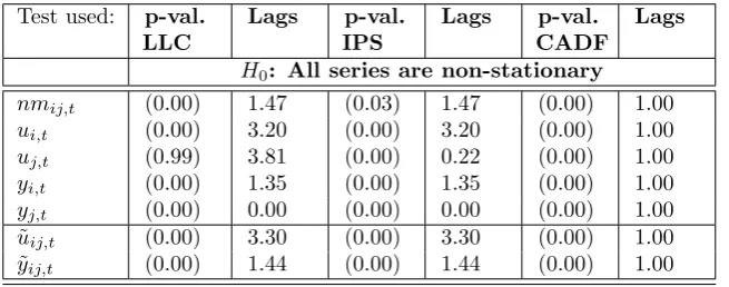
unemployment rate the Levin-Lin-Chu test could not reject the null of non-stationarity. However, the LLC-test rejects the null hypothesis of an integrated time series if the unemployment rate is transformed into regional differences (˜uij,t). Thus, given the overall

picture presented by the panel unit root tests it seems reasonable to handle the variables as stationary processes so that we can also run regressions in levels (as it is the case for Blundell-Bond System GMM) without running the risk of spurious regression results. The estimation results are reported in the next section.

<<< Table 4 about here >>>

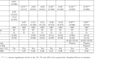
For estimation we start from an unrestricted presentation of the baseline model inclu-ding the core labour market variables real income (y) and unemployment rates (u) and test for parameter constraints according to eq.(9) and eq.(10). As the results in table 5 show for almost all model specifications the null hypothesis for equal parameter cannot be rejected on the basis of standard Wald tests. Compared to the the static specification in column 2, the (relative) RMSE criterion of the model strongly increases if we add a dynamic component to the migration equation. The RSME for each equation is thereby computed as the ratio compared to the RMSE of the static POLS benchmark specification in column 1. As discussed above the POLS, REM and FEM estimators are biased for dy-namic panel data models. We thus compute a corrected FEM specification as proposed e.g. in Kiviet (1995) as well as the Arellano-Bond (1991) und Blundell-Bond (1998) system GMM estimators. According to the relative RMSE criterion the Blundell-Bond system GMM specification has the smallest forecast error. The coefficients for labour market signals are statistically significant and of expected signs. Moreover the SYS-GMM speci-fication passes standard tests for autocorrelation in the residuals (m1 and m2 statistic) as well as the Hansen J-statistic for instrument validity. The reported C-statistic for the exogeneity of the instruments in the level equation shows the validity of the augmented approach in extension to the standard Arellano-Bond first differenced model.

<<< Table 5 about here >>>

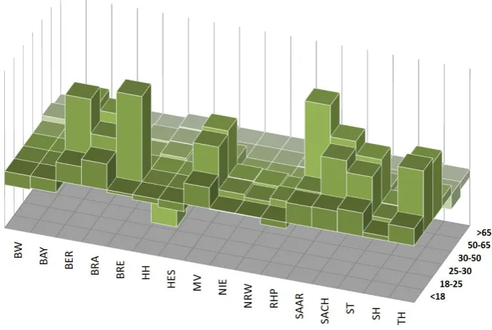
degree of migratory interregional immobility was found to coexist with large regional labour market disparities. Fachin (2007) and Etzo (2007) report similar results to hold for Italian South-North migration trends, while Alecke & Untiedt (2000) as well as Alecke et al. (2010) identify such effects for German East-West migration throughout the 1990s. However, the latter study found that along with a second wave of East-West movements in early 2000 net flows out of East Germany on the contrary were much higher than expected after controlling for its weak labour market and macroeconomic performance. Since this trend was accompanied by a gradual fading out of economic distortions, this supports the view of ”repressed” migration flows for that period. As the result in table 6 show for the period 1996 to 2006 we find a statistically significant positive East German dummy, which indicates higher net in-migration balances for the East German Spatial Planning Regions than their labour market performance would suggest. To get further insights we also estimate a specification which includes Federal state level fixed effects. The results for the state dummies in the baseline model are reported in table 7 (column 1) and are graphically shown in figure 7. The fixed effects for federal states, which represent remaining time-fixed macro regional influential factors for the regional net in-migration rate, are statistically significant for many cases.

<<<Table 6 and table 7 about here >>>

<<< Figure 7 about here >>>

As the figure highlights, for all six East German state dummies we get statistically significant and positive coefficients. Negative coefficients are found for the West German states Baden Wuerttemberg, Bavaria and Hessen. A Wald test for joint effect of the set of state dummies turns out to be highly significant. For both models (including the East German dummy and the set of state dummies), the impact of labour market variables is of expected sign and higher than in the baseline specification.

lower net in-migration rates relative to benchmark category Type 1 (highly agglomerated area with regional urban center above 100,000 persons and population density above 300 inhabitants/sqm). This may hint at the role played by regional centers of agglomeration in attracting migration flows and may be interpreted in favour of a ’reurbanisation’ process in Germany for the period 1996 to 2006. Similar trends were also reported in Swiaczny et al. (2008).10 _{Finally, testing for the effects of regional human capital endowments and}

international competitiveness shows mixed results. While the proxy for the latter variable in terms of foreign turnover relative to total turnover in manufacturing sector industries shows the expected positive effect on net in-migration, the regional endowment with hu-man capital is insignificant. This finding corresponds to recent results for Spain between 1995–2002, where regional differences in human capital do not help to explain migration flows (see Maza & Villaverde, 2004). The latter may be explained by the fact that not the region specific stock of human capital but rather the individual endowment of the prospective migrant is the appropriate level of measurement. However, the latter variable is not observable for regional data.

In order to check for the appropriateness of our augmented SYS-GMM specifications, we perform a variety of of postestimation tests for instrument appropriateness, temporal and cross-sectional dependence of the error term. The test results are reported in table 6. With respect to IV appropriateness and temporal autocorrelation of the error terms, all model specifications shows satisfactory results. In order to control for cross-sectional error dependence due to unobserved common factors, we first add year dummies to our model specification, which also turn out to be jointly significant. We then apply the Sargan’s difference test for the SYS-GMM model (CCDGM M) as described above, which tests for

the nature of the cross-sectional dependence given unobserved common factors as being homogeneous our heterogeneous among regions. In order to run the test, we first need to judge whether the set of explanatory variables (excluding instruments for the lagged endogenous variable) is exogenous with respect to the combined error term. This can be easily tested by means of a Sargan/Hansen J-statistic based overidentification test. As the results in table 6 show, only those model specification which include fixed state effects pass the overidentification test for the vector of explanatory variables. For these equations we could then apply CCDGM M from eq.(16) in order to test for the existence of

hetero-geneous factor loading for the common factor structure of the error terms as proposed by Sarafidis et al. (2009). The test results do not indicate any sign of misspecification after including period-fixed effects for standard significance levels. In sum, the augmented

neoclassical migration equation shows to be an appropriate representation of the data generating process and highlights the role of key labour market variables in explaining net in-migration rates for German Spatial Planning regions.

7

Sensitivity analysis: Disaggregate estimates by age groups

Given the supportive findings for the neoclassical migration model at the aggregate level, we finally aim to check for the sensitivity of the results when different disaggregated age groups are used. Detailed results for the baseline and augmented specification of the migration model are shown in table A.1 and table A.2 in the appendix.11_{We are especially}

interested to analyse whether the estimated coefficients for the labour market signals change for different age-groups. Indeed, the results show that the migratory response to labour market variables is much higher for workforce relevant age groups. The resulting coefficient size for real income and unemployment rate differences together with 95 % confidence intervals for the estimated models are plotted in figure 8 and 9.

<<< Figure 8 and Figure 9 about here >>>

The coefficient for real income differences in figure 8 shows a clear inverted U-shape when plotted for the different age-groups in ascending order. While for migrants up to 18 year real income difference do not seem to matter, especially for migrants with an age between 18 to 25 years and 25 to 30 years the estimated coefficient is statistically significant and much higher compared to the overall migration equation from table 6. For older age-groups the effect reduces gradually. The results are found to be very similar for the baseline and augmented migration specification (see figure 8). Similar results were found for regional unemployment rate differences, which are found to be almost equally important for age groups until 50 years and only show much smaller and partly insignifi-cant coefficient signs for elderly age groups. If we look at the distribution of the state-level fixed effects for each estimated age-group specification, the estimation results show that the positive dummy variable coefficients for the East German states particularly hold for the workforce relevant age groups. The results are graphically shown in figure 10 for the baseline migration model (detailed results for the estimated coefficients of the baseline and augmented specification are reported in the the appendix).

<<< Figure 10 about here >>>

Finally, table 8 computes the ’relative importance’ of the labour market variables by age-groups with respect to net migration flows. Thereby, the relative importance refers to the quantification of an individual regressors contribution to a multiple regression model (see e.g. Groemping, 2006, for an overview). This allows us to further answer the question, in how far our estimation results support the prominent role of labour market conditions in guiding internal migration rates (of the workforce population) in Germany. Table 8 calculates to specifications either based on the squared correlation of the respective regressor with the dependent variables (univariate R2_{, specification A) as}

well as the standardized estimated SYS-GMM coefficents from the augmented migration model in table A.2. This latter metric for assessing the relative importance of regressors has the advantage over the simple benchmark in specification A since it accounts for the correlation of regressors. As the table shows both methods assign a significant share for the two key labour market variables in predicting migration flows, especially for the workforce population (up to 50 % joint contribution in Specification A for age-group 18 to 25 years and even up to 65 % for age-group 25 to 30 years in Specification B). The SYS-GMM thereby on average assigns a stronger weight to real income differences in explaining net in-migration relative to unemployment differences. However, the overall picture confirms our interpretation of the regression tables in assigning a prominent role to labour market imbalances in driving German internal migration.

<<< Table 8 about here >>>

8

Conclusion

results of the standard neoclassical migration model remain stable if commuting flows, the regional human capital endowment, the region’s international competitiveness as well as differences in the settlement structure are added as further explanatory variables. The inclusion of the regional net in-commuting rate shows a negative correlation with migra-tion underlying the substitutive nature of the two variables. Also, an increasing level of international competitiveness attracts further in-migration flows. We also find hetero-geneity for different types of regional settlement structure proxied by population density and we observe structural differences for the two East-West macro regions (by including individual federal state level fixed effects or an combined East German dummy). We finally estimate the migration model for age-group specific subsamples of the data. Here the impact of labour market signals is found to be of greatest magnitude for workforce relevant age-groups (18 to 25, 25 to 30 and 30 to 50 years). This latter result underlines the prominent role played by labour market conditions in guiding internal migration rates of the working age population in Germany.

References

[1] Ahn, S.; Schmidt, P. (1995): ”Efficient estimation of models for dynamic panel data”, in: Journal of Econometrics, Vol. 68, pp. 5-27.

[2]Alecke, B.; Mitze, T.; Untiedt, G. (2010): ”Internal Migration, Regional Labour Market Dynamics and Implications for German East-West-Disparities - Results from a Panel VAR”, in: Jahrbuch f¨ur Regionalwissenschaft (online first).

[3]Alecke, B.; Untiedt, G. (2000): ”Determinanten der Binnenwanderung in Deutsch-land seit der Wiedervereinigung”, Working Paper, University of M¨unster.

[4] Arellano, M. (1989): ”A Note on the Anderson-Hsiao Estimator for Panel Data”, in: Economic Letters, Vol. 31, pp.337-341.

[5]Arellano, M.; Bond, S. (1991): ”Some tests of specification for panel data: Monte Carlo evidence and an application to employment equations”, in: Review of Economic Studies, Vol. 58, pp. 277-297.

[6] Arellano, M.; Bover, O. (1995): ”Another look at the instrumental-variable esti-mation of error-components models”, in: Journal of Econometrics, Vol. 68, pp. 29-52.

[8] Baltagi, B.; Bresson, G.; Pirotte, A. (2007): ”Panel unit root tests and spatial dependence”, in: Journal of Applied Econometrics, Vol. 22(2), pp. 339-360.

[9]Baltagi, B.; Blien, U.; Wolf, K. (2007): ”Phillips Curve or Wage Curve? Evidence from West Germany 1980-2004”, IAB Discussion paper No. 14/2007.

[10] Blanchflower, D.G.; Oswald, A.J. (1994): ”The Wage Curve”, MIT Press,

Cambridge MA.

[11] Blundell, R.; Bond, S. (1998): ”Initial conditions and moment restrictions in dynamic panel data models”, in: Journal of Econometrics, Vol. 87, pp. 115-143.

[12] Bond, S.; Hoeffler, A.; Temple, J. (2001): ”GMM Estimation of Empirical

Growth Models”, CEPR Discussion Paper No. 3048.

[13] B¨uchel, F.; Schwarze, J. (1994): ”Die Migration von Ost- nach Westdeutschland - Absicht und Realisierung”, in: Mitteilungen aus der Arbeitsmarkt- und Berufsforschung, 27 (1), pp.43-52.

[14] Burda, M.C. (1993): ”The determinants of East-West German migration. Some first results”, in: European Economic Review, Vol. 37, pp.452-461.

[15] Burda, M.C.; H¨ardle, W.; M¨uller, M.; Werwartz, A. (1998): ”Semiparame-tric Analysis of German East-West Migration Intentions: Facts and Theory”, in: Journal of Applied Econometrics, Vol. 13, pp.525-541.

[16] Burda, M.C.; Hunt, J. (2001): ”From Reunification to Economic Integration: Productivity and the Labour Market in East Germany”, in: Brookings Papers on Econo-mic Activity, Issue 2, pp.1-92.

[17] Br¨ucker, H.; Tr¨ubswetter, P. (2004): ”Do the Best Go West? An Analysis of the Self-Selection of Employed East-West Migrants in Germany”, IZA Discussion Papers 986.

[18] Decressin, J. (1994): ”Internal Migration in West Germany and Implications for East-West Salary Convergence”, in: Weltwirtschaftliches Archiv, Vol. 130, pp.231-257.

[19] Devillanova, C.; Garcia-Fontes, W. (2004): ”Migration across Spanish Provin-ces: Evidence from the Social Security Records (1978-1992)”, in: Investigaciones Econo-micas, Vol. 28(3), pp.461-487.

[20] Eichenbaum, M.; Hansen, L.; Singelton, K. (1988): ”A Time Series Analysis of Representative Agent Models of Consumption and Leisure under Uncertainty”, in: Quarterly Journal of Economics, Vol. 103, pp.51-78.

[22] Everaert, G.; Pozzi, L. (2007): ”Bootstrap-based bias correction for dynamic panels”, in: Journal of Economic Dynamics and Control, Vol. 31(4), pp. 1160-1184.

[23] Fachin, S. (2007): ”Long-run Trends in Internal Migrations in Italy: A Study on Panel Cointegration with Dependent Units”, in: Journal of Applied Econometrics, Vol. 51, No. 4, pp.401-428.

[24] Ghatak, S.; Mulhern, A.; Watson, J. (2008): ”Inter-regional migration in

transition economies: the case of Poland”, in: Review of Development Economics, Vol. 12(1), pp. 209-222.

[25] Greenwood, M.J.; Hunt, G.L.; Rickman, D.S.; Treyz, G.I. (1991):

”Mi-gration, Regional Equilibrium, and the Estimation of Compensating Differentials”, in:

American Economic Review, Vol. 81, pp.1382-1390.

[26] Gr¨omping, U. (2006): ”Relative Importance for Linear Regression in R: The Package relaimpo”, in: Journal of Statistical Software, Vol. 17, Issue 1, pp. 1-27.

[27] Hatzius, J. (1994): ”Regional Migration, Unemployment and Vacancies: Evidence from West German Microdata”, Applied Economics Discussion Paper Series Nr. 164, University Oxford.

[28] Harris, J.R.; Todaro, M.P. (1970): ”Migration, Unemployment and

Develop-ment: A Two Sector Analysis”, in: American Economic Review, Vol. 60, pp.126-142.

[29] Holtz-Eakin, D.; Newey, W.; Rosen, H.S. (1988): ”Estimating vector autore-gressions with panel data”, in: Econometrica, Vol. 56, pp. 1371-1395.

[30] Holtz-Eakin, D. (1994): ”Public sector capital and the productivity puzzle”, in: Review of Economics and Statistics, Vol. 76, pp. 12-21.

[31] Hunt, J. (2000): ”Why Do People Still Live in East Germany?”, NBER Working Paper No. 7645.

[32] Im, K.; Pesaran, M.; Shin, Y. (2003): ”Testing for unit roots in heterogeneous panels”, in: Journal of Econometrics, Vol. 115, pp. 53-74.

[33] Jackman, R.; Savouri, S. (1992): ”Regional Migration in Britain: An Analysis of Gross Flows Using NHS Central Register Data”, in: Economic Journal, Vol. 102 (415), pp.1433-1450.

[34] Kiviet, J. (1995): ”On bias, inconsistency, and efficiency of various estimators in dynamic panel data models”, in: Journal of Econometrics, Vol. 68(1), pp. 53-78.

[36] Munnel, A. (1992): ”Infrastructure Investment and Economic Growth”, in: Jour-nal of Economic Perspectives, Vol. 6(4), pp. 189-198.

[37] Napolitano, O.; Bonasia, M. (2010): ”Determinants of different internal migra-tion trends: the Italian experience”, MPRA Paper No. 21734.

[38] Nickell, S. (1981): ”Biases in Dynamic Models with Fixed Effects”, in: Econome-trica, Vol. 49, pp.1417-1426.

[39] Parikh, A.; Van Leuvensteijn, M. (2003): ”Interregional labour mobility, ine-quality and wage convergence”, in: Applied Economics, Vol. 35, pp.931-941.

[40] Pesaran, M.H. (2006): ”Estimation and Inference in Large Heterogeneous Panels with a Multifactor Error Structure”, in: Econometrica, Vol. 74(4), pp. 967-1012.

[41] Pesaran, M.H. (2007): ”A simple panel unit root test in the presence of cross-section dependence”, in: Journal of Applied Econometrics, Vol. 22(2), pp. 265-312.

[42] Pissarides, C.; McMaster, I. (1990): ”Regional Migration, Wages and Unem-ployment: Empirical Evidence and Implications for Policy”, in: Oxford Economic Papers, Vol. 42, pp.812-831.

[43] Puhani, P.A. (2001): ”Labour Mobility - An Adjustment Mechanism in

Euro-land?”, in: German Economic Review, Vol. 2(2), pp. 127-140.

[44] Rainer, H.; Siedler, T. (2009): ”Social networks in determining migration and labour market outcomes: Evidence from the German Reunification”, in: Economics of Transition, Vol. 17, Issue 4, pp. 739-767.

[44] Roodman, D. (2006): ”How to Do xtabond2: An introduction to ’Difference’ and ’System’ GMM in Stata”, Center for Global Development, Working Paper No. 103.

[45] Sarafidis, V.; Wansbeek, T. (2010): ”Cross-sectional Dependence in Panel Data Analysis”, MPRA Paper No. 20367.

[46] Sarafidis, V.; Robertson, D. (2009): ”On the impact of error cross-sectional dependence in short dynamic panel estimation”, in: Econometrics Journal, Vol. 12(1), pp. 62-81.

[47]Sarafidis, V.; Yamagata, T.; Robertson, D. (2009): ”A test of cross section de-pendence for a linear dynamic panel model with regressors”, in: Journal of Econometrics, Vol. 148(2), pp. 149-161.

[49] Schwarze, J. (1996): ”Beeinflusst das Lohngef¨alle zwischen Ost- und Westdeutsch-land das Migrationsverhalten der Ostdeutschen?”, in: Allgemeines Statistisches Archiv, Vol. 80 (1), pp.50-68.

[50] Sevestre, P.; Trognon, A. (1995): ”Dynamic Linear Models”, in: Matyas, L.; Sevestre, P. (Eds.): ”The Econometrics of Panel Data. A Handbook of the Theory with Applications”, 2.Edition, Dordrecht et al.

[51] Silva, S.; Hadri, K.; Tremayne, A. (2009): ”Panel Unit Root Tests in the

Presence of Cross-Sectional Dependence: Finite Sample Performance and an Application ”, in: Econometrics Journal, Vol. 12, Issue 2, pp. 340-366.

[52] Sjaastad, L. (1962): ”The Costs and Returns of Human Migration”, in: The

Journal of Political Economy, Vol.70, pp. 80-93.

[53] Swianczy, Graze, P.; Schl¨omer, C. (2008): ”Spatial Impacts of Demographic Change in Germany. Urban Population Processes Reconsidered”, in: Zeitschrift f¨ur Bevl-kerungswissenschaft, Vol. 33, pp. 181-205.

[54] Todaro, M. (1969): ”A Model for Labor Migration and Urban Unemployment in Less Developed Countries”, in: American Economic Review, Vol. 59(1), pp. 138-148.

[55] Wagner, G. (1992): ”Arbeitslosigkeit, Abwanderung und Pendeln von Arbeits-kr¨aften der neuen Bundesl¨ander”, in: Sozialer Fortschritt, pp.84-89.

[56] Westerlund, O (1997): ”Employment Opportunities, Wages and International

Migration in Sweden 1970-1989”, in: Journal of Regional Science, Vol. 37, pp.55-73.

Table 1: Variable definition and data sources

Variable Description Source

NM Net migration defined as in- minus outmigration German Statistical Office NM(to18) Net migration for persons under 18 years German Statistical Office NM(18to25) Net migration for persons between 18 and 24 years German Statistical Office NM(25to30) Net migration for persons between 25 and 29 years German Statistical Office NM(30to50) Net migration for persons between 30 and 49 years German Statistical Office NM(50to65) Net migration for persons between 50 and 65 years German Statistical Office NM(over65) Net migration for persons 65 years and above German Statistical Office POP Population Level VGRdL

Y Gross Domestic Product (real) per Person VGRdL

UR Unemployment Rate Federal Employment Agency COMM Net Commuting level defined as in- minus

outcommuting

German Statistical Office HK Human Capital level defined as %-share of

employees with university degree relative to total employees

German Statistical Office

INTCOMP International Competitiveness proxied by foreign turnover relative to total turnover in manufacturing industries

German Statistical Office

EAST Binary dummy variable for regions in East Germany

own calculation STATE Set of binary dummies for each of the 16 Federal

States

own calculation TIME Set of year specific time dummies for sample period

1996 to 2006

own calculation SETTLE Set of binary dummies for types of settlement

structure with:

Federal Institute for Research on Building, Urban Affairs and Spatial Development (BBSR) Type1: Highly agglomerated area with regional

urban center above 100.000 persons and population density above 300 inhabitants/sqm

Type2: Highly agglomerated area with regional urban center above 100.000 persons and population density below 300 inhabitants/sqm

Type3: Agglomerated area with population density above 200 inhabitants/sqm

Type4: Agglomerated area with regional urban center above 100.000 persons and population density between 100-200 inhabitants/sqm

Type5: Agglomerated area without regional urban center above 100.000 persons and population density between 150-200 inhabitants/sqm

Type6: Rural area with population density above 100 inhabitants/sqm

Type7: Rural area with population density below 100 inhabitants/sqm

i index for regioni(region in focus)

j index for regionj (rest of the country aggregate)

Table 2: Descriptive statistics for continuous variables in the sample

Variable Obs. Mean Std. Dev. Min Max Unit

INM 1067 0.00 7.21 -95.90 37.01 in 1000 persons INM (to18) 1067 0.00 1.91 -24.41 32.41 in 1000 persons INM (18to25) 1067 0.00 1.85 -12.97 15.76 in 1000 persons INM (25to30) 1067 0.00 1.27 -9.93 12.42 in 1000 persons INM (30to50) 1067 0.00 2.48 -30.99 8.24 in 1000 persons INM (50to65) 1067 0.00 0.91 -10.61 1.82 in 1000 persons INM (over65) 1067 0.00 0.62 -7.05 1.23 in 1000 persons POP 1067 848.10 607.13 226.29 3466.52 in 1000 persons Y 1067 51.23 7.49 34.02 80.01 in 1000 Euro UR 1067 11.84 4.94 4.37 26.18 in % COMM 873 -33.49 37.44 -177.73 36.31 in 1000 persons HK 873 7.30 2.71 2.88 16.81 in % INTCOMP 946 30.05 11.42 0.82 61.12 in %

Table 3: Descriptive statistics for binary variables in the sample

Variable Obs. % with

X = 1

EAST 1067 23.7

Federal State Level Dummies

BW 1067 12.4 BAY 1067 18.5 BER 1067 1.0 BRA 1067 5.2 BRE 1067 1.0 HH 1067 1.0 HES 1067 5.1 MV 1067 4.1 NIE 1067 13.4 NRW 1067 13.4 RHP 1067 5.1 SAAR 1067 1.0 SACH 1067 5.1 ST 1067 4.1 SH 1067 5.1 TH 1067 4.1

Settlement Type Dummies

Type1 1067 15.5 Type2 1067 15.5 Type3 1067 17.5 Type4 1067 17.5 Type5 1067 8.2 Type6 1067 15.4 Type7 1067 10.3

Note: BW = Baden-Wurttemberg, BAY = Bavaria, BER = Berlin, BRA = Brandenburg, BRE = Bremen, HH = Hamburg, HES = Hessen, MV = Mecklenburg-Vorpommern, NIE = Lower Saxony, NRW = North

Figure 1: Spatial Distribution of Net In-Migration Flows for German Regions

Figure 1: 1996

Figure 4: Spatial Distribution of Real Income in German Regions

Figure 6: Regional Settlement Structure by Size of Urban Centres and Population Density

Note:

Type1 = Highly agglomerated area with regional urban center above 100.000 persons and population density above 300 inhabitants/sqm

Type2 = Highly agglomerated area with regional urban center above 100.000 persons and population density below 300 inhabitants/sqm

Type3 = Agglomerated area with population density above 200 inhabitants/sqm

Type4 = Agglomerated area with regional urban center above 100.000 persons and population density between 100-200 inhabitants/sqm

Type5 = Agglomerated area without regional urban center above 100.000 persons and population density between 150-200 inhabitants/sqm

Type6 = Rural area with population density above 100 inhabitants/sqm Type7 = Rural area with population density below 100 inhabitants/sqm

Table 4: Results of Panel unit root tests for variables in the migration model

Test used: p-val. LLC

Lags p-val. IPS

Lags p-val. CADF

Lags

H0: All series are non-stationary

nmij,t (0.00) 1.47 (0.03) 1.47 (0.00) 1.00

ui,t (0.00) 3.20 (0.00) 3.20 (0.00) 1.00

uj,t (0.99) 3.81 (0.00) 0.22 (0.00) 1.00

yi,t (0.00) 1.35 (0.00) 1.35 (0.00) 1.00

yj,t (0.00) 0.00 (0.00) 0.00 (0.00) 1.00

˜

uij,t (0.00) 3.30 (0.00) 3.30 (0.00) 1.00

˜

yij,t (0.00) 1.44 (0.00) 1.44 (0.00) 1.00

Table 5: Baseline Specifications of the Neoclassical Migration Model for German Spatial Planning Regions

Dep. Var.: nmij,t POLS POLS POLS REM FEM FEMc AB-GMM SYS-GMM

nmij,t−1 0.90∗∗∗ 0.90∗∗∗ 0.78∗∗∗ 0.92∗∗∗ 0.84∗∗∗ 0.88∗∗∗

(0.011) (0.011) (0.022) (0.031) (0.001) (0.001)

ui,t−1 -0.74∗∗∗

(0.114)

uj,t−1 0.64∗

(0.399) ˜

uij,t−1 -0.72∗∗∗ -0.05 -0.05 -0.32∗∗ -0.28∗ -0.53∗∗∗ -0.19∗∗∗

(0.114) (0.041) (0.041) (0.166) (0.166) (0.023) (0.006)

yi,t−1 0.07

(0.315)

yj,t−1 -0.14

(0.378) ˜

yij,t₋1 0.07 0.12 0.12 -0.26 -0.10 0.25∗∗∗ 0.03∗∗

(0.314) (0.108) (0.112) (0.372) (0.374) (0.066) (0.014)

No. of obs. 1067 1067 1067 1067 1067 1067 1067 1067

No. of groups 97 97 97 97 97 97 97 97

No. of years 11 11 11 11 11 11 11 11

βui =−βuj (0.83) (0.60 (0.42) (0.11) (0.19) (0.00) (0.14)

βyi =−βyj (0.76) (0.60) (0.24) (0.39) (0.59) (0.58) (0.14)

m1 andm2 (0.42)/(0.24) (0.35)/(0.24)

J-Stat. Overall Passed Passed

C-Stat. LEV-EQ Passed

Time Dummies (11) No Yes Yes Yes Yes Yes Yes Yes

Relative RMSE 1 1.07 0.38 0.38 0.41 0.39 0.43 0.38

Note: ***, **, * = denote significance levels at the 1%, 5% and 10% level respectively. Standard Errors in brackets.

Figure 7: State level effects for German States in the Aggregate Baseline Migration Model

Note: For details of calculation see table 7.

Figure 10: State level effects Effects in Baseline Migration Model by States and Age

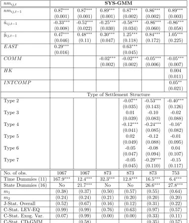
Table 6: Augmented Neoclassical Migration Model for German Spatial Planning Regions

nmij,t SYS-GMM

nmij,t−1 0.87∗∗∗ 0.87∗∗∗ 0.89∗∗∗ 0.87∗∗∗ 0.86∗∗∗ 0.89∗∗∗

(0.001) (0.001) (0.001) (0.002) (0.002) (0.003) ˜

uij,t−1 -0.33∗∗∗ -0.52∗∗∗ -0.25∗∗∗ -0.58∗∗∗ -0.86∗∗∗ -0.86∗∗∗ (0.008) (0.022) (0.030) (0.034) (0.060) (0.058) ˜

yij,t−1 0.47∗∗∗ 0.48∗∗∗ 0.30∗∗∗ 1.25∗∗∗ 0.84∗∗∗ 1.05∗∗∗

(0.046) (0.11) (0.047) (0.118) (0.172) (0.225)

EAST 0.29∗∗∗ _0.63∗∗∗

(0.016) (0.045)

COM M -0.02∗∗∗ _-0.02∗∗∗ _-0.05∗∗∗ _-0.05∗∗∗

(0.002) (0.002) (0.006) (0.007)

HK 0.004

(0.011)

IN T COM P 0.05∗∗

(0.021) Type of Settlement Structure

Type 2 -0.07∗∗ _-0.53∗∗∗ _-0.40∗∗∗

(0.035) (0.143) (0.126)

Type 3 0.01 -0.10 -0.02

(0.039) (0.083) (0.088) Type 4 -0.12∗∗∗ _-0.24∗∗∗ _-0.16∗

(0.041) (0.085) (0.082)

Type 5 0.02 -0.12 -0.01

(0.049) (0.088) (0.095)

Type 6 -0.05 -0.08 0.04

(0.047) (0.094) (0.107) Type 7 -0.05 -0.29∗∗∗ _-0.15

(0.045) (0.110) (0.117) No. of obs. 1067 1067 873 873 873 753 Time Dummies (11) 167.9∗∗∗ _12.4∗∗∗ _32.3∗∗∗ _12.8∗∗∗ _16.5∗∗∗ _6.4∗∗∗

State Dummies (16) No 21.7∗∗∗ _{No No 26.6}∗∗∗ _27.8∗∗∗

m1 (0.38) (0.37) (0.50) (0.57) (0.55) (0.64)

m2 (0.24) (0.24) (0.21) (0.20) (0.20) (0.20) J-Stat. Overall (0.52) (0.67) (0.16) (0.12) (0.31) (0.22) C-Stat. LEV-EQ (0.99) (0.99) (0.76) (0.63) (0.97) (0.57) C-Stat. Exog. Var. (0.07) (0.99) (0.00) (0.00) (0.33) (0.11) C-Stat. CD-GMM (0.58) (0.35) (0.57)

Table 7: Estimated state level effects in Migration Models

Model: Baseline Augmented

BW -0.22∗∗∗ _-0.27∗∗∗

(0.023) (0.079)

BAY -0.18∗∗∗ _-0.39∗∗∗

(0.019) (0.119)

BER 0.42∗∗ _1.12∗∗∗

(0.188) (0.264)

BRA 0.38∗∗∗ _0.63∗∗∗

(0.045) (0.137)

BRE 0.20 1.23∗∗

(0.255) (0.492)

HH -0.18 1.08∗

(0.346) (0.553)

HES -0.15∗∗∗ _-0.32∗∗

(0.030) (0.125)

M V 0.34∗∗∗ _0.53∗∗∗

(0.045) (0.125)

N IE -0.02 -0.05 (0.021) (0.105)

N RW -0.03 0.02 (0.026) (0.059)

RHP -0.09∗∗∗ _-0.67∗∗∗

(0.023) (0.129)

SAAR -0.01 -0.49 (0.254) (0.583)

SACH 0.37∗∗∗ _0.79∗∗∗

(0.052) (0.174)

ST 0.33∗∗∗ _0.23∗

(0.047) (0.133)

SH 0.06∗∗ _0.07

(0.024) (0.107)

T H 0.32∗∗∗ _0.19

(0.037) (0.154)

Note: ***, **, * = denote significance levels at the 1%, 5% and 10% level respectively. BW =

Baden-Wurttemberg, BAY = Bavaria, BER = Berlin, BRA = Brandenburg, BRE = Bremen, HH = Hamburg, HES = Hessen, MV = Mecklenburg-Vorpommern, NIE = Lower Saxony, NRW = North Rhine-Westphalia, RHP = Rhineland-Palatine, SAAR = Saarland, SACH = Saxony, ST = Saxony-Anhalt, SH =

Figure 8: Coefficients for Real Income Differences (y˜ij,t−1) by Age Groups

Note: For details of calculation see table A.1 and table A.2. Dotted lines are 95 % convidence intervals.

Figure 9: Coefficients for Unemployment Rate Differences (u˜ij,t−1) by Age Groups

Table 8: Relative Contribution of Labour Market Variables in Explaining Migration Flows

Specification A Specification B

Age-Group yij,t−1 uij,t−1 Joint yij,t−1 uij,t−1 Joint Up to 18 1 % 3 % 4 % 0 % 19 % 19 % 18 to 25 29 % 21 % 50 % 19 % 8 % 27 % 25 to 30 18 % 14 % 31 % 54 % 11 % 65 % 30 to 50 1 % 5 % 6 % 5 % 8 % 13 % 50 to 65 1 % 1 % 1 % 2 % 0 % 2 % Over 65 1 % 0 % 2 % 1 % 1 % 2 %

Note: Specification A is based on the computation of the squared correlation of the respective regressor with the dependent variables (univariateR2). Specification B is calculated using the estimated SYS-GMM coefficent from the augmented migration model specification in table A.2. The estimation coefficient for regressorxkis further

standardized as ˆβstandardized,k= ˆβk

√_s kk

√_syy, whereskk andsyydenote the empirical variances of regressorxkand

the dependent variableyrespectively. As long as one only compares regressors within models for the samey, division by√_s

Table A.1: Baseline Migration Model based on System GMM Estimation

nmij,t To18 18to25 25to30 30to50 50to65 Over65

nmij,t−1 0.87∗∗∗ 0.86∗∗∗ 0.86∗∗∗ 0.87∗∗∗ 0.90∗∗∗ 0.88∗∗∗

(0.001) (0.005) (0.004) (0.002) (0.001) (0.002) ˜

uij,t−1 -0.78∗∗∗ -0.91∗∗∗ -0.78∗∗∗ -0.42∗∗∗ 0.19∗∗∗ -0.03 (0.044) (0.156) (0.148) (0.036) (0.019) (0.018) ˜

yij,t−1 0.28∗∗ 3.73∗∗∗ 4.03∗∗∗ 0.25∗∗ -0.83∗∗∗ -0.59∗∗∗ (0.112) (0.406) (0.395) (0.102) (0.042) (0.043)

BW -0.31∗∗∗ _-0.35∗∗∗ _-0.37∗∗∗ _-0.17∗∗∗ _0.11∗∗∗ _0.01

(0.035) (0.093) (0.093) (0.018) (0.016) (0.011)

BAY -0.28∗∗∗ _-0.21∗∗∗ _-0.20∗∗∗ _-0.15∗∗∗ _0.07∗∗∗ _-0.01

(0.031) (0.075) (0.077) (0.018) (0.016) (0.009)

BER 0.42∗∗∗ _1.67∗∗ _{1.32 0.12 -0.17}∗∗∗ _-0.02

(0.144) (0.721) (0.937) (0.187) (0.054) (0.068)

BRA 0.59∗∗∗ _0.89∗∗∗ _1.12∗∗∗ _0.36∗∗∗ _-0.24∗∗∗ _-0.06∗∗∗

(0.044) (0.171) (0.156) (0.052) (0.019) (0.018)

BRE -0.06 1.95∗∗∗ _{-0.38 -0.03 0.04 -0.10}∗∗∗

(0.256) (0.610) (0.470) (0.161) (0.107) (0.133)

HH -0.11 -0.12 -1.22 -0.12 0.07 0.09 (0.410) (0.712) (1.133) (0.018) (0.125) (0.160)

HES -0.18∗∗∗ _-0.22∗ _-0.27∗∗ _-0.12∗∗∗ _0.09∗∗∗ _0.03

(0.045)) (0.133) (0.110) (0.018) (0.031) (0.027)

M V 0.48∗∗∗ _1.11∗∗∗ _1.19∗∗∗ _0.26∗∗∗ _-0.31∗∗∗ _-0.12∗∗∗

(0.047) (0.171) (0.164) (0.051) (0.022) (0.021)

N IE -0.01 0.14∗∗ _0.15∗∗ _{-0.02 -0.05}∗∗∗ _-0.04∗∗∗

(0.020) (0.065) (0.057) (0.017) (0.011) (0.007)

N RW -0.01 0.08 0.13∗ _{-0.02 -0.01 -0.01}

(0.035) (0.065) (0.071) (0.019) (0.010) (0.008)

RHP -0.14∗∗∗ _{0.15 0.08 -0.08}∗∗∗ _{0.02 -0.04}∗∗∗

(0.035) (0.102) (0.089) (0.017) (0.026) (0.014)

SAAR 0.46 0.49 2.20∗∗ _{0.07 0.11 0.03}

(0.384) (0.764) (1.062) (0.153) (0.176) (0.082)

SACH 0.47∗∗∗ _1.33∗∗∗ _1.49∗∗∗ _0.24∗∗∗ _-0.33∗∗∗ _-0.15∗∗∗

(0.055) (0.194) (0.177) (0.052) (0.028) (0.022)

ST 0.53∗∗∗ _1.06∗∗∗ _1.17∗∗∗ _0.25∗∗∗ _-0.35∗∗∗ _-0.15∗∗∗

(0.088) (0.177) (0.178) (0.051) (0.020) (0.021)

SH 0.10∗∗∗ _0.18∗ _0.19∗∗∗ _0.07∗∗∗ _0.07∗∗∗ _0.03

(0.030) (0.094) (0.056) (0.013) (0.013) (0.007)

T H 0.39∗∗∗ _1.42∗∗∗ _1.31∗∗∗ _0.21∗∗∗ _-0.34∗∗∗ _-0.18∗∗∗

(0.058) (0.212) (0.173) (0.048) (0.019) (0.018) No. of obs. 1067 1067 1067 1067 1067 1067 Time Dummies (11) Yes Yes Yes Yes Yes Yes

Note: ***, **, * = denote significance levels at the 1%, 5% and 10% level respectively. BW =

Baden-Wurttemberg, BAY = Bavaria, BER = Berlin, BRA = Brandenburg, BRE = Bremen, HH = Hamburg, HES = Hessen, MV = Mecklenburg-Vorpommern, NIE = Lower Saxony, NRW = North Rhine-Westphalia, RHP = Rhineland-Palatine, SAAR = Saarland, SACH = Saxony, ST = Saxony-Anhalt, SH =