Bankruptcy prediction models: How to choose the most relevant variables?

Munich Personal RePEc Archive

Bankruptcy prediction models: How to

choose the most relevant variables?

du Jardin, Philippe

Edhec Business School

January 2009

du Jardin, P., 2009, Bankruptcy prediction models: How to choose the most relevant variables? Bankers, Markets & Investors, issue 98, January-February, pp. 39–46.

1

Bankruptcy Prediction Models:

How to Choose the Most Relevant Variables?

Philippe du Jardin Professor

Edhec Business School 393, Promenade des Anglais

BP 3116 06202 Nice Cedex 3

Email : philippe.dujardin@edhec.edu

Abstract – This paper is a critical review of the variable selection methods used to build empirical bankruptcy prediction models. Recent decades have seen many papers on modelling techniques, but very few about the variable selection methods that should be used jointly or about their fit. This issue is of concern because it determines the parsimony and economy of the models and thus the accuracy of the predictions. We first analyze those variables that are considered the best bankruptcy predictors, then present variable selection and review the main variable selection techniques used to design financial failure models. Finally, we discuss the way these techniques are commonly used, and we highlight the problems that may occur with some non-linear methods.

2

1 Introduction

Bankruptcy prediction has given rise to an extensive body of literature since the late 1960’s, the aim of which is to assess the determinants of financial failure and to design prediction rules. Beginning with Altman (1968) and continuing through Agarwal and Taffler (2008), nearly all factors that may strongly influence the accuracy of a model have been analyzed through empirical research. Ample supporting evidence may be found in the literature, which provides insights into the issues regularly emerging in this field (Balcaen and Ooghe, 2006). However, a comprehensive examination of the main research topics shows that they have not received the same degree of attention. We have analyzed 190 papers on bankruptcy prediction models written in the last forty. They focus largely on five major issues:

• first (46% of studies), modelling techniques: the aim is to provide an in-depth understanding of the ability of classification and regression methods to create accurate models (Altman, 1968; Ohlson, 1980; Odom and Sharda, 1990…). More than fifty methods have been used (discriminant analysis, logistic regression, neural networks, support vector machine, rules induction, spline regression, rough sets, gambler’s ruin model, hazard model, probit, learning vector quantization, regression tree, and so on);

• second (23%), explanatory variables: the aim is to find the best predictors in terms of model accuracy (Keasey and Watson, 1987; Mossman et al., 1998…). As there is no theory of financial failure or of the variables to use, the strategy involves mining data to find empirical predictors that may perform well in predicting the bankruptcy of a sample of firms;

• third (11%), types of failure a model is able to forecast: since many models are designed to classify only two groups (bankrupt vs. non-bankrupt), some researchers have attempted to develop multi-state models (i.e., multiple states of financial health), such as models able to predict a final bankruptcy resolution (liquidation, reorganization, takeover by another firm: Kumar et al., 1997…), events that may affect the financial or economic health of companies (omission or reduction of dividend payments, default on loan payments: Altman et al., 1994…), or to estimate the financial situation of a firm (distress, insolvency, vulnerability, unsound health: Platt and Platt, 2002…);

• fourth (7%), the factors that may influence the accuracy of a model: sample size, relative size of each group (bankrupt vs. non-bankrupt) in a sample, time period during which the data are collected, cost of misclassification, forecast timeframe (Karels and Prakash, 1987…); • fifth (barely 6%), analysis of uncommon variable selection techniques: the aim is to use techniques other than those commonly used in an attempt to overcome some of the limitations imposed by univariate statistical tests and some methods whose evaluation criteria are optimized for a discriminant analysis or a logistic regression (Back et al., 1994; Sexton et al., 2003; Brabazon and Keenan, 2004…);

• finally, and marginally, a few other issues have been tackled: some authors have analyzed how useful a theoretical model of the firm may be in the design of bankruptcy models (Gentry et al., 1987; Aziz et al., 1988…); others have looked into the conditions of replicability of existing models (Moyer, 1977; Grice and Dugan, 2003…). Still others have attempted to identify bankruptcy or failure processes or to build sector- (bank, insurance) or category-based models (publicly quoted companies, small companies: Barniv and Hershbarger, 1990…).

It is clear then that variable selection has been somewhat neglected. A “good” model is able to generalize properly and thus to provide accurate results with data not used in its design. To generalize, it must be as parsimonious as possible; that is, the number of adjustable free parameters, and especially the number of variables, should be as low as possible. Variable selection, and variable selection techniques, are thus of great importance.

3

of variable selection, an analysis of the methods commonly used to develop corporate failure models, and a discussion of the way these methods are used.

The paper is essentially concerned with two major questions that crop up during variable selection: what variables will form the initial pool of variables on which the model will ultimately draw? What method should be used for the final selection?

The content of the paper is organized as follows: in section 2, we describe the main factors that may explain financial failure and we propose a classification of explanatory variables that best reflect these factors. This section outlines the main explanatory predictors of financial failure as considered by the authors of bankruptcy models. In section 3, we introduce the variable selection issue, while describing existing methods, then we evaluate the characteristics and assumptions of the selection techniques actually used. In this section, we present a hierarchy of selection methods and evaluate the fit with commonly used modelling techniques. And, in section 4, we point out some important future research topics in this field.

2 Bankruptcy factors and explanatory variables

2.1 Bankruptcy factors

The causes of bankruptcy are numerous, as many authors have pointed out (Argenti, 1976; Lussier, 1995; Blazy and Combier, 1997; Sullivan et al., 1998; Bradley, 2004). The typology suggested by Blazy and Combier (1997) offers a relevant synthesis of these major causes: • accidental causes: malfeasance, death of the leader, fraud, disasters, litigation…;

• market problems: loss of market share, failure of customers, inadequate products…; • financial threats: under-capitalization, cost of capital, default on payment, loan refusal…; • information and managerial problems: incompetency, prices and stocks, inadequate organization…;

• macroeconomic factors of fragility: declining demand, increased competition, credit rationing, high interest rates…;

• costs and production structure: excessive labour costs, over- or under-investment, sudden loss of a supplier, inadequate production process…;

• strategy: failures of major projects, acceptance of unprofitable markets.

Financial problems, then, have many causes, and these causes are easily determined. But finding the variables that may reflect these factors is altogether different. Indeed, each cause identified above cannot be entirely reduced to a single, measurable parameter. So what then are the variables that act as indicators of these vulnerabilities?

First, most of these causes are predictable over time and their inertia is such that they are potentially preventable. Second, a thorough reading of financial and accounting documents can detect almost all of them; in other words, their symptoms are observable (Pérez, 2002). It is for this reason that financial documents are the main source of information when designing bankruptcy models. However, the likelihood of failure cannot be modelled efficiently by relying on financial indicators alone; to guarantee that the phenomenon is approached in its entirety, it is necessary to take into account other parameters, whether they are easily measured or not.

2.2 Variables that best reflect company failure

The variables that best reflect all these factors fall into one or more of three main categories: • the first has to do with the company itself and it includes both financial variables (balance sheet or income statement variables) and variables that represent its main characteristics: structure, management, strategy, products…;

4

• the third, not directly linked to the above analysis, has to do with financial markets and information related to the way these markets evaluate a company’s risk of failure. It relies on the hypothesis of market efficiency, for which a stock price or a stock return reflects future expected cash flows of a firm and as a consequence may be viewed as a proxy for its financial health. For this reason, several authors recommend using this proxy to complement or to replace other types of variables.

All explanatory variables used by bankruptcy models come from these three sources. They may be constructed using different kinds of data, as shown in table 1.

Table 1: Typology of explanatory variables commonly used by bankruptcy prediction models

Variables Frequency (decreasing order) of use in the 190 studies 1 Financial ratio (ratio of two financial variables) 93%

2 Statistical variable (mean, standard deviation, variance, logarithm, factor analysis scores…

calculated with ratios or financial variables) 28% 3 Variation variable (evolution over time of a ratio or a financial variable) 14%

4 Non-financial variable (any characteristic of a company or its environment other than those related to its financial situation)

13%

5 Market variable (ratio or variable related to stock price, stock return) 6%

6 Financial market variable (data coming a balance sheet, an income statement or any financial

documents) 5%

The total is greater than 100 as several types of variables may have been used at the same time.

2.2.1 Financial ratios

5

Moreover, over 53% of these studies include only ratios in their models and almost 78% include ratios used either alone or in conjunction with another type of variable

2.2.2 Other types of variables

Aside from ratios, there are five other types of variables that play secondary roles that are not, all the same, entirely negligible. “Statistical variables”, in second place on our list, are any kind of transformation of specific ratios or financial variables by statistical or mathematical functions: mean, standard deviation, variance, logarithm… They also include factor analysis scores. These computations are often used to standardize the data: one of the main standardization strategies, in fact, is to compute the logarithm of “financial variables”. Since Altman (1968), as it happens, the logarithm of the variable “total assets” has been considered one of the variables with real discriminatory power.

“Variation variables”, the third most frequently used category, are for the most part year-on-year changes to a ratio or financial variable. They embody a dynamic vision of failure that assumes that the process of failure may take more than one form and that trends or variations alone may reveal the phase of the process in which the firm finds itself. This representation cannot replace a static one, but it can complement it: a static representation can detect an imbalance, while a dynamic one will show its direction.

“Non-financial variables” are in fourth place. They include qualitative or quantitative characteristics of firms1 _{other than accounting ones, or of their environment.}2 _{They are part of}

a strategy to broaden the dimensions of failure to include those dimensions that cannot be included in accounting models but that nonetheless play a significant role.

“Financial market variable”, in fifth place, reflect the financial value of companies as estimated by financial markets, on the basis of their stock price or stock return.

Finally, in sixth place, we find “financial variables”, especially those used to compute financial ratios, which may be used alone, without being standardized, such as liquidity variables, computed with cash flow indicators, or asset and turnover variables.

2.2.3 Financial ratios: the most commonly used variables

Financial ratios are the most commonly used variables because of their economic character, not because of their absolute predictive ability. Indeed, the data used to compute financial ratios are easy to collect and check, while non-accounting data can sometimes be collected for only some types of firms or not at all; financial markets data, for instance, are available only for publicly quoted companies.

Too few studies dealing with the predictive ability of these variables have been done for us to account for the frequency with which they are used. Back et al. (1994) showed that a model built with financial ratios alone may perform better than a model built with common financial variables (assets, debt, income). Mossman et al. (1998) analyzed the results obtained with ratio-based models and financial market variable-based models and concluded that the former had slightly better results than the latter. Keasey and Watson (1987) compared results obtained with three different models to determine whether a model including non-financial variables, either alone or in conjunction with financial ratios, would make better predictions than a model based solely on ratios. The model using financial and non-financial indicators led to better results than the two others, and the ratio-based model was a bit more accurate than the model based on non-financial variables. Lussier (1995) considered the problem of building a bankruptcy model with qualitative variables that described both the leaders and the

1 _{Leaders’ characteristics, long-term strategy, number of partners, customer concentration, relationship with}

banks, market share, age of the firm, size, sector, and so on.

6

business of firms, but the model was not satisfactory, since the rate at which it correctly identified sound firms came only to 73% and the rate at which it identified bankrupt firms was barely 65%. Atiya (2001) compared a ratio-based model with a ratio and financial market variable-based model and concluded that the ratio-based model was slightly more accurate than the competing model. Tirapat and Nittayagasetwat (1999) developed a model composed of financial ratios and macro-economic variables intended to take into account the influence of environmental factors on companies. Barely more than 70% of its predictions were accurate. As far as the “variation variables” are concerned, Pérez (2002) did a study of several samples of small and medium-sized firms and achieved far better results with absolute figures than with data describing the variation of financial variables. Her findings were consistent with those obtained by Pompe and Bilderbeek (2005), who conclude that absolute values of ratios are better predictors than are the changes over time.

So far there are too few points of comparison to account with certainty for the popularity of financial ratios, although we may well imagine the reasons. As ratios provide excellent forecast ability, the marginal cost of using other variables, what with their relatively high cost, puts them out of the picture.

3 Variable selection

As discussed above, financial ratios are the most commonly used indicators in bankruptcy prediction models. However, there is a huge number of ratios that have proven to have good predictive ability. Our literature review shows that in the last forty years more than 500 different ratios have been used to build models. This figure includes only those variables that were selected to create models, not those that were initially considered but failed to make the final cut.

Choosing a subset of variables from an initial set is essential to the development of a model. First of all, it is essential to the parsimony of the model because, as we mentioned above, generalization requires parsimony, and parsimony is directly related to the number of variables included in a model. It is also essential for the accuracy of the model because, generally, not all variables contribute equally to its performance. Some may be less informative, others noisy, meaningless, correlated and thus redundant, or irrelevant. The aim of a selection process is therefore to find a subset of relevant variables for a given problem, composed of elements as independent as possible, and sufficiently numerous to account for the problem.

3.1 Variable selection: a non-monotonic problem

Variable selection remains difficult because it is often non-monotonic. Indeed, the best subset of p variables rarely includes the best subset of q variables, where q < p. If it did, a sequential search, adding or removing variables one at a time, would easily lead to a solution. Moreover, the best subset does not exist in itself; instead, it depends heavily on the method used to design the model (inductive algorithm), although these two steps are usually taken separately. Faced with this non-monotonic character, only an exhaustive search of all possible combinations will lead to the best subset(s). But the resulting combinatorial explosion, even with fairly small problems (i.e., fewer than ten variables), makes these searches impossible. It is for that reason that most methods rely on heuristic procedures that do a limited search in the space of all combinations.

These heuristic procedures are made up of three basic elements (Dash and Liu, 1997):

• a search procedure that explores a subspace of all possible combinations and generates a set of candidate solutions;

7

3.2 Selection methods

3.2.1 Search procedure

As mentioned above, not all problems lend themselves to an exhaustive search. In these circumstances, thus when the evaluation criterion is non-monotonic and the search space is too large (for n variables, there are 2n - 1 possible subsets), it is better to explore only a limited part of the variable space. On the other hand, when the monotonic hypothesis is borne out, wider exploration is possible. Several classifications of methods have been suggested in the literature. Dash and Liu (1997) propose breaking them down into three families:

• “complete” methods: these methods may find an optimal solution if the evaluation criterion is monotonic. The search is said to be “complete” and “non-exhaustive” because it does not evaluate all possible combinations; instead, it uses heuristic functions to reduce the search space without jeopardizing the chances of finding the best subset for the evaluation criteria used (Branch and Bound);

• “heuristic” or sequential methods: these methods are used to relax the monotonicity assumption that the methods above impose on the evaluation criterion. They are characterized by way they explore the variable space: some start with an empty set of variables, then add them one at a time (forward search); other ones start with all variables, then remove them, also one at a time (backward search). They are easy to use and produce results quickly, but they lead to non-optimal solutions because they search only a part of the space and are unable to backtrack to a previous stage: once a variable is selected, it cannot be removed (nesting). To improve this procedure, some methods alternate forward and backward steps (stepwise) but computing time increases as the search space expands (Plus l – Take Away r, floating methods…);

• “random” methods: unlike the previous methods, which are deterministic, these methods lead to solutions that depend heavily on initial conditions. They start by choosing at random a set of variables, and then search using one of two strategies: either sequential – therefore identical to those described above – such as Simulated Annealing, or random, such as genetic algorithms.

Sequential or random methods are the most useful because the problems are often non-monotonic and a single analysis of the individual characteristics of a set of variables cannot evaluate the characteristics of the set itself.

3.2.2 Evaluation criterion

Once a search procedure has chosen a subset of variables, this subset must be evaluated. For a classification task, such as the one we are dealing with here, the evaluation will focus on its ability to discriminate between groups. We must therefore find a criterion that will be used, finally, to compare different subsets and select the one or those that will offer the best results. John et al. (1994) divide the evaluation methods into two categories: those for which the evaluation relies solely on the intrinsic characteristics of the data without using the inductive algorithm (filter methods), and those that do rely on the performance of the inductive algorithm when using the variables that are to be evaluated (wrapper methods). The criteria used by these methods are as follows:

8

• dependent criteria: with these criteria, the inductive algorithm is used during the evaluation process. For instance, only those variables that lead to the lowest generalization error will be selected. Wrappers often achieve good results because the selected subsets are well suited to the inductive method, but they always require significant computing time.

For the classification problems considered in this paper, independent criteria such as Wilks’s lambda or likelihood statistics are among the measures often used to select variables.

3.2.3 Stopping criterion

Without a suitable stopping criterion, a selection process could run indefinitely. Many criteria may be used to interrupt a search. Most of the time these criteria take the form of a maximum number of iterations, a predefined number of variables, the absence of improvement after addition or removal of variables, or the achievement of optimal predictive ability (in other words, an acceptable generalization error). These criteria depend on computation heuristics and sometimes on statistical tests. Finally, the search is stopped once no additional variable is considered relevant.

3.3 Selection methods used to build bankruptcy prediction models

When developing business failure models, researchers usually use a two-step procedure to choose to include the “best” variables in their models. Initially, general considerations (financial, empirical, and so on) are used to identify a large set of variables, but only a few are finally chosen, often for statistical reasons.

The initial set, often made up of a few dozen variables, is most often identified without using any automatic process; instead, it is arbitrarily chosen based on the popularity of the variables in the literature or on their predictive ability as assessed in previous studies. This “historical” set was built on the strength of the seminal work done by researchers who, in the 1930’s, first assessed the usefulness of financial ratios as a means of predicting corporate failure and by those who contributed to an understanding of the role played by multivariate statistical methods in the field of bankruptcy prediction. Among these latter researchers are Altman (1968), Odom and Sharda (1990), Zmijewski (1984) and Zavgren (1985). All of this work may be viewed as the initial step towards the elaboration of a comprehensive set of essential bankruptcy predictors, which has been complemented over the years by other variables, whether they are accounting-based measures of the financial health of a firm or not.

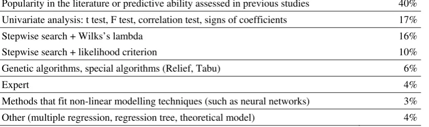
The final set, on the other hand, is selected in three of five cases with automatic procedures, whereas in the other cases all variables initially selected are finally used to design models. The main criteria used to make these selections in the 190 studies we have reviewed are shown in table 2 (below).

Table 2: Criteria used to select explanatory variables to include in bankruptcy models

Popularity in the literature or predictive ability assessed in previous studies 40% Univariate analysis: t test, F test, correlation test, signs of coefficients 17% Stepwise search + Wilks’s lambda 16% Stepwise search + likelihood criterion 10% Genetic algorithms, special algorithms (Relief, Tabu) 6%

Expert 4%

Methods that fit non-linear modelling techniques (such as neural networks) 3% Other (multiple regression, regression tree, theoretical model) 4%

9

the final models because their discrimination ability has been verified either by financial analysis or empirical studies. However, there is no guarantee that variables that have proven reliable bankruptcy indicators in some circumstances will always be so in others. For instance, when confronted with samples other than those used to design them, all the studies that attempt to test the behaviour of models such as Altman’s (1968) or Ohlson’s (1980) come to the same conclusion: original models always achieve poor results, and even when their coefficients are re-estimated, the results are weaker than those obtained with the original values (Moyer, 1977; Grice and Dugan, 2003). This is a result of the characteristics of the variables, which are contingent. It is for this reason that, when building a new model, it is always better to seek ad hoc variables. Bardos (1995) points out that there are indicators with general, permanent discriminatory ability that can reveal risk when they worsen (liquidity, solvability, reimbursement ability, production costs, leverage), but that only large forces that account for bankruptcy are permanent, and that variables that reflect these forces are contingent and may change over time.

17% of studies used univariate statistical tests that measure only the individual discrimination ability of single variables. It has long been known (Altman, 1968) that, once included in a model, variables with high individual power of discrimination may not perform well or not as well as another set composed of variables that do not show strong individual discrimination ability. There are two reasons for this phenomenon. First, an evaluation criterion for variables is never completely independent of the modelling techniques in use: a variance criterion, such as Wilks’s lambda, is well suited to discriminant analysis, and a likelihood criterion is well suited to logistic regression. So there is no reason to assume that these criteria will perform well with other classification methods. But that is precisely the assumption that many authors have made. Second, selecting variables on the basis of a single test for differences between means implies a failure to allow for the possible interaction of these variables, interaction that could detract from the predictive quality of some variables and add to that of others. As a consequence, some variables may be selected even though they perform poorly together, and others, which could have made for a good model, may be discarded. Alongside selections done by univariate tests, we see that 16% of studies use a stepwise method with a Wilks’s Lambda criterion and 10% also use a stepwise search but with a likelihood criterion as an evaluation measure. Strangely, despite a great diversity of search procedures and of evaluation functions or criteria, researchers always use the same methods: as discriminant analysis and logistic regression are the most widely used modelling techniques, the variable selection methods remain the same.

Finally, 17% use other means: 6% use genetic algorithms, 4% ask an expert to choose their variables, 3% use selection techniques designed for non-linear methods, and 4% use marginal means (multiple regression, classification tree, theoretical models of the firm).

These results show that only 35% of the studies use an effective variable selection strategy (stepwise method, genetic algorithms or techniques for non-linear models), whereas 65% of the studies often rely on either history or univariate statistical tests to choose variables, when, given the issues described in the introduction, a more rigorous protocol would have been advisable.

These results also show something else which does not appear prima facie. Roughly 50 studies (26%) use discriminant analysis as a major modelling method or as a benchmark, 40 (21%) use logistic regression for the same purpose and 75 (39%) use a special kind of method, called neural networks;3 the 25 remaining studies rely on less widely used methods

3 _{Most neural networks used in this field are in the Multilayer Perceptron family. This class of networks is able}

10

(genetic algorithms, rough set, Bayesian model, hazard model, support vector machine, regression tree…). When we analyze the variable selection strategies and the modelling techniques used with them, we see that discriminant analysis and logistic regression are sometimes used with sub-optimal variable selection criteria, even if the fit of these criteria and the modelling techniques is not wrong. By contrast, when a neural network is used to create models, the fit with the selection technique is barely acceptable. Indeed, 75 of the 190 studies used this modelling method: of these 75, 32 selected the variables for neural models on the basis of their popularity in the financial literature, 24 on the basis of univariate statistical tests or criteria optimized for discriminant analysis or logistic regression, six with a genetic algorithm, four with a technique that fits neural networks, and nine with other means. However, Leray and Gallinari (1998) have stated that since many parametric variable selection methods rely on the hypothesis that input-output variable dependence is linear or that input variable redundancy is well measured by the linear correlation of these variables, such methods are clearly ill-suited to non-linear methods, and hence to neural networks, because the latter are non-linear. In such situations, it is better to use methods suitable for non-linear techniques, or methods that do not rely on these assumptions, such as genetic algorithms. As a consequence, the authors of neural models who used univariate statistical tests that are supposed to evaluate the discriminatory ability of variables, or evaluation criteria such as Wilks’s lambda, have chosen inadequate parameters that may have led to the selection of useless variables as well as to the removal of variables of interest. Very little research has used either a genetic algorithm (Back et al., 1994; Sexton et al., 2003; Brabazon and Keenan, 2004…) or a suitable technique to take into account the characteristics of neural networks. Nevertheless, in each case, the experiments were done with few variables, small samples, and without attempting comparisons of several methods or criteria, thus reducing the significance of their results. Only one study (Back et al., 1996) has compared a pair of sets of variables optimized for a discriminant analysis, a logistic regression and a neural network, but this comparison was made simply to analyze the differences between the models in terms of accuracy over different prediction timeframes (one, two or three years). This extensive body of work shows that too many authors of bankruptcy models use variable selection methods without considering the characteristics of the modelling techniques.

4 Conclusion

Several conclusions may be drawn from this review. First, many studies have undertaken to explore the suitability of regression or classification methods as viable techniques for the creation of bankruptcy prediction models. However, this focus has led to a neglect of other problems, in particular that of variable selection, as if choosing variables to design a model were a secondary task. Today, we know a lot about the performance of modelling techniques and their use. We also know that the accuracy of a model is in part the result of the intrinsic characteristics of the modelling technique and in part that of the fit of this technique and the variable selection procedure involved in its design. It is therefore worth to notice that many authors strongly recommend comparing the results obtained with different classification or regression techniques but do not apply the same reasoning to the selection methods that will choose the variables relied on by these techniques. Greater attention should be paid to this issue. Second, many studies show that both financial ratios and a probability of bankruptcy behave in a non-linear manner and that it is hardly possible to develop accurate models as long as this linearity cannot be taken into account. It is for that reason that further exploration of non-linear models designed with ad hoc variables would not be unwelcome.

11

Finally, beyond the prediction issue, exploration of opportunities offered by selection techniques should be undertaken in directions other than those related to model design. This exploration would, for instance, allow a better understanding of the determinants of failure and help answer the following question: are there or are there not any “strong”, sample- and method-independent variables that reflect failure factors? With its analysis of failure from multiple angles and its identification of patterns, it would, in short, help account for the dynamic side of financial failure.

12

References

Agarwal, V., Taffler, R. (2008), “Comparing the Performance of Market-based and Accounting-based Bankruptcy Prediction Models”, Journal of Banking and Finance, vol. 32, n° 8, pp.

1541-1551.

Altman, E. I. (1968), “Financial Ratios, Discriminant Analysis and the Prediction of Corporate Bankruptcy”, Journal of Finance, vol. 23, n° 4, pp. 589-609.

Altman, E. I., Marco, G., Varetto, F. (1994), “Corporate Distress Diagnosis: Comparisons Using Linear Discriminant Analysis and Neural Network – The Italian Experience”,

Journal of Banking and Finance, vol. 18, n° 3, pp. 505-529.

Argenti, J. (1976), Corporate Collapse: the Causes and Symptoms, Halsted Press, Wiley,

New York.

Atiya, A. F. (2001), “Bankruptcy Prediction for Credit Risk Using Neural Networks: A Survey and New Results”, IEEE Transactions on Neural Networks, vol. 12, n° 4, pp. 929-935.

Aziz, A., Emanuel, D. C., Lawson, G. C. (1988), “Bankruptcy Prediction: An Investigation of Cash Flow Based Models”, Journal of Management Studies, vol. 25, n° 5, p. 419-437.

Back, B., Laitinen, T., Sere, K., Van Wezel, M. (1996), “Choosing Bankruptcy Predictors Using Discriminant Analysis, Logit Analysis and Genetic Algorithms”, Turku Centre for Computer Science, Technical Report, n° 40.

Back, B., Oosterom, G., Sere, K., Van Wezel, M. (1994), “A Comparative Study of Neural Networks in Bankruptcy Prediction”, Proceedings of the 10th Conference on Artificial Intelligence Research in Finland, Finnish Artificial Intelligence Society, pp. 140-148.

Balcaen, S., Ooghe, H. (2006), “35 Years of Studies on Business Failure: An Overview of the Classical Statistical Methodologies and their Related Problems”, British Accounting Review, vol. 38, n° 1, pp. 63-93.

Bardos, M. (1995), “Détection précoce des défaillances d’entreprises à partir des documents comptables”, Bulletin de la Banque de France, Supplément Études, 3ème trimestre, pp. 57-71.

Barniv, R., Hershbarger, A. (1990), “Classifying Financial Distress in the Life Insurance Industry”, Journal of Risk and Insurance, vol. 57, n° 1, pp. 110-136.

Blazy, R., Combier, J. (1997), “La défaillance d'entreprise : causes économiques, traitement judiciaire et impact financier”, Economica.

Brabazon, A., Keenan, P. B. (2004), “A Hybrid Genetic Model for the Prediction of Corporate Failure”, Computational Management Science, Special Issue, vol. 1, n° 3-4, pp. 293-310.

Bradley, D. B. (2004), “Small Business: Causes of Bankruptcy, Small Business Advancement National Center”, University of Central Arkansas, College of Business Administration, Research Paper.

Dash, M., Liu, H. (1997), “Feature Selection for Classification”, Intelligent Data Analysis,

vol. 1, n° 3, pp. 131-156.

Gentry, J. A., Newbold, P., Whitford, D. T. (1987), “Funds Flow Components, Financial Ratios and Bankruptcy”, Journal of Business Finance and Accountancy, vol. 14, pp. 595-606.

Grice, J. S., Dugan, M. T. (2003), “Reestimations of the Zmijewski and Ohlson Bankruptcy Prediction Models”, Advances in Accounting, vol. 20, pp. 77-93.

Gupta, M. C. (1969), “The Effect of Size, Growth, and Industry on The Financial Structure of Manufacturing Companies”, Journal of Finance, vol. 24, n° 3, pp. 517-529.

Horrigan, J. O. (1983), “Methodological Implications of Non-Normally Distributed Financial Ratios Factors Associated with Insolvency amongst Small Firms”, Journal of Business Finance and Accounting, vol. 10, n° 4, pp. 683-689.

John, G. H., Kohavi, R, Pfleger, K. (1994), “Irrelevant Features and the Subset Selection Problem”, in Machine Learning: Proceedings of the 11th International Conference, New

13

Karels, G. V., Prakash, A. J. (1987), “Multivariate Normality and Forecasting of Business Bankruptcy”, Journal of Business Finance and Accounting, vol. 14, n° 4, pp. 573-593.

Keasey, K., Watson, R. (1987), “Non-Financial Symptoms and the Prediction of Small Company Failure : A Test of Argenti's Hypothesis”, Journal of Business Finance and Accounting, vol. 14, n° 3, pp. 335-354.

Kumar, N., Krovi, R., Rajagopalan, B. (1997), “Financial Decision Support with Hybrid Genetic and Neural Based Modeling Tools”, European Journal of Operational Research, vol. 103,

n° 2, pp. 339-349.

Leray, P., Gallinari, P. (1998), “Feature Selection with Neural Networks”, Behaviormetrika,

vol. 26, n° 1, pp.145-166.

Lev, B., Sunder, S. (1979), “Methodological Issues in the Use of Financial Ratios”, Journal of Accounting and Economics, vol. 1, n° 3, pp. 187-210.

Lussier, R. N. (1995), “A Nonfinancial Business Success versus Failure Prediction Model for Young Firms”, Journal of Small Business Management, vol. 33, n° 1, pp. 8-20.

Mossman, C. E., Bell, G. G., Swartz, L. M., Turtle, H. (1998), “An Empirical Comparison of Bankruptcy Models”, Financial Review, vol. 33, n° 2, pp. 35-53.

Moyer, R. C. (1977), “Forecasting Financial Failure: A Re-Examination”, Financial Management, vol. 6, n° 1, pp. 11-17.

Odom, M. C., Sharda, R. (1990), “A Neural Network Model for Bankruptcy Prediction”,

Proceedings of the IEEE International Joint Conference on Neural Networks, San Diego,

California, vol. 2, pp. 163-168.

Ohlson, J. A. (1980), “Financial Ratios and the Probabilistic Prediction of Bankruptcy”,

Journal of Accounting Research, vol. 18, n° 1, pp. 109-131.

Pérez, M. (2002), De l’analyse de la performance à la prévision de défaillance : les apports de la classification neuronale, Thèse de doctorat, Université Jean-Moulin, Lyon III.

Platt, H. D., Platt, M. B. (2002), “Predicting Corporate Financial Distress: Reflections on Choice-Based Sample Bias”, Journal of Economics and Finance, vol. 26, n° 2, pp. 184-199.

Pompe, P. P. M., Bilderbeek, J. (2005), “The Prediction of Bankruptcy of Small- and Medium-Sized Industrial Firms”, Journal of Business Venturing, vol. 20, n° 6, pp. 847-868.

Salmi, T., Martikainen, T. (1994), “A Review of the Theoretical and Empirical Basis of Financial Ratio Analysis”, Finnish Journal of Business Economics, vol. 4, n° 94, pp. 426-448.

Sexton, R. S., Sriram, R. S., Etheridge, H. (2003), “Improving Decision Effectiveness of Artificial Neural Networks: A Modified Genetic Algorithm Approach”, Decision Sciences,

vol. 34, n° 3, pp. 421-442.

Sullivan, T. A., Warren, E., Westbrook, J. (1998), “Financial Difficulties of Small Businesses and Reasons for their Failure”, U.S. Small Business Administration, Working Paper, n° SBA-95-0403.

Tirapat, S., Nittayagasetwat, A. (1999), “An Investigation of Thai Listed Firms’ Financial Distress Using Macro and Micro Variables”, Multinational Finance Journal, vol. 3, n° 2, pp. 103-125.

Zavgren, C. V. (1985), “Assessing the Vulnerability to Failure of American Industrial Firms: A Logistic Analysis”, Journal of Business Finance and Accounting, vol. 12, n° 1, pp. 19-45.