Evaluation of Different Classification Techniques for
WEB Data
Chitra Nasa
M.Tech CSE Deptt Hindu College of engg.
.Sonepat, Haryana
Suman
A.P CSE Deptt Hindu College of engg.
Sonepat, Haryana
ABSTRACT
The growth of data-mining applications such as classification and clustering has shown the need for machine learning algorithms to be applied to large scale data. In this paper we present the comparison of different classification techniques using Waikato Environment for Knowledge Analysis or in short, WEKA. WEKA is open source software which consists of a collection of machine learning algorithms for data mining tasks. The aim of this paper is to examine the performance of different classification methods for a set of large data. The algorithm which have been tested are J48, SMO, Part, OneR, ZeroR and Navies Bayes Algorithm. The Syskill and webert we page rating data [11] with a total data of 1660 and a dimension of 332 rows and 5columns will be used to test and validate the differences between the classification methods or algorithms.
Keywords
Machine Learning, Data Mining, WEKA, Classification, Web data, web mining.
1. INTRODUCTION
The basic idea of our work is to examine the performance of different classification methods using WEKA for Web Data. A major problem in Web data analysis is loss of focus on important information because lots of ambiguity is there in Web information. To reach at a highly rated web page, normally, many searches generally involve the clustering or classification of large scale data. All of these test procedures are said to be necessary in order to reach the ultimate concentrated page which is the desire of a user. However, before reaching at an informative page which gives lots of information to user, he reaches at a spider of web where lots of unnecessary information is also present along with the useful information. This kind of difficulty could be resolved with the aid of machine learning which could be used directly to obtain the end result with the aid of several artificial intelligent algorithms which perform the role of classifiers. Machine learning covers such a wide range of processes that it is difficult to define precisely. A dictionary definition includes phrases such as to gain knowledge or understanding of skill by studying the instruction or experience. The extraction of important information from a large heap of data and its correlations is often the advantage of using machine learning. Newknowledge about tasks is constantly being discovered by humans and vocabulary changes. There is aconstant stream of new events in the world and continuing redesign of Artificial Intelligent systems to conform to new knowledge is impractical but machine learning methods might be able to track much of it.
There is a significant amount of study with machine learning algorithm such as Bayes Network, J48 Decision tree and Part, ZeroR, OneR and SMO Algorithm.
2. METHODS
Classification [1] is a data mining task of predicting the value of a categorical variable (target or class) by building a model based on one or more numerical and/or categorical variables (predictors or attributes).
2.1
J48 Decision Tree
- A decision tree partitions the input space of a data set into mutually exclusive regions, each of which is assigned a label, a value or an action to characterize its data points. The decision tree mechanism is transparent and we can follow a tree structure easily to see how the decision is made [2]. A decision tree is a tree structure consisting of internal and external nodes connected by branches. An internal node is a decision making unit that evaluates a decision function to determine which child node to visit next. The external node, on the other hand, has no child nodes and is associated with a label or value that characterizes the given data that leads to its being visited. However, many decision tree construction algorithms involve a two - step process. First, a very large decision tree is grown. Then, to reduce large size and overfiting the data, in the second step, the given tree is pruned. The pruned decision tree that is used for classification purposes is called the classification tree [3]. To build a decision tree, we need to calculate entropy and information gain [2] –E(S) = ∑
Information Gain The information gain is depending on the decrease in entropy after a dataset is split on a selected attribute. Constructing a decision tree is mean to find an attribute which possess the highest information gain value
Gain( ) ( ) ( ) Algorithm: Generate decision tree. Generate a decision tree
from the training tuples of data partition D.
35 Output: A decision tree.
Figure 1: Decision Tree Algorithm
2.2
Navies Bayes Classifier
Bayesian networks are a powerful probabilistic representation, and their pridictors [4] or attributes. In particular, the naive Bayes classifier is a Bayesian network where the class has no parents and each attribute has the class as its sole parent.
The Naive Bayesian classifier is based on Bayes’ theorem with independence assumptions between predictors. A Naive Bayesian model is easy to build, with no complicated iterative parameter estimation which makes it particularly useful for very large datasets. Despite its simplicity, the Naive Bayesian classifier often does surprisingly well and is widely used because it often outperforms more sophisticated classification methods.
Algorithm Bayes [5] theorem provides a way of calculating the posterior probability, P(c|x), from P(c), P(x), and P(x|c). Naive Bayes classifier assumes that the effect of the value of a predictor (x) on a given class (c) is independent of the values of other predictors. This assumption is called class conditional independence.
posterior prob. likelihood prior prob.
( | ) ( | ) ( )
( )
prior probability of predictor
( | ) ( | ) ( | ) ( | ) ( )
P(c|x) is the posterior probability of class (target) given predictor (attribute).
P(c) is the prior probability of class.
P(x|c) is the likelihood which is the probability of predictor given class.
P(x) is the prior probability of predictor.
2.3
SMO Classifier
–Sequential minimal optimization (SMO) is an algorithm for efficiently solving the optimization problem which arises during the training of support vector machines. It was invented by John Platt in 1998 at Microsoft Research. SMO [6] is widely used for training support vector machines and is implemented by the popular libsvm tool. The publication of the SMO algorithm in 1998 has generated a lot of excitement in the SVM community, as previously available methods for SVM training were much more complex and required expensive third-party QP solvers.
SMO is an iterative algorithm for solving the optimization problem described above. SMO breaks this problem into a series of smallest possible sub-problems, which are then solved analytically. Because of the linear equality constraint involving the Lagrange multiplier, the smallest possible problem involves two such multipliers.
The algorithm proceeds as follows:
Find a Lagrange multiplier that violates the Karush–Kuhn–Tucker (KKT) conditions for the optimization problem.
Pick a second multiplier and optimize the pair. Repeat steps 1 and 2 until convergence.
When all the Lagrange multipliers assure the KKT conditions, the problem has been solved. Although this algorithm is guaranteed to converge, heuristics are used to choose the pair off of multipliers so that it can accelerate the rate of convergence.
2.4 ZeroR Classifier
ZeroR is the simplest classification method which relies on the target and ignores all predictors .ZeroR classifier [7] simply predicts the majority category (class). Although there is no predictability power in ZeroR, it is useful for determining a baseline performance as a benchmark for other classification methods. Algorithm Construct a frequency table for the target and select its most frequent value. Predictors Contribution There is nothing to be said about the predictors contribution to the model because ZeroR does not use any of them.
Model Evaluation The ZeroR only predicts the majority class correctly. As mentioned before, ZeroR is only useful for determining a baseline performance for other classification methods.
2.5 OneR Classifier
OneR, short for "One Rule", is a simple, yet accurate, classification algorithm that generates one rule for each predictor in the data, and then selects the rule with the smallest total error as its "one rule". To create a rule for a predictor, we have to construct a frequency table for each predictor against the target. OneR Algorithm [8] for each predictor, For each value of that predictor, make rule as follows-
Count how often each value of target(class) appears
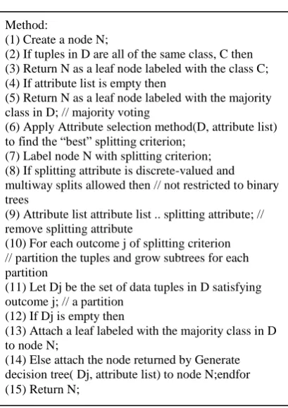
Find the most frequent class Method:
(1) Create a node N;
(2) If tuples in D are all of the same class, C then (3) Return N as a leaf node labeled with the class C; (4) If attribute list is empty then
(5) Return N as a leaf node labeled with the majority class in D; // majority voting
(6) Apply Attribute selection method(D, attribute list) to find the “best” splitting criterion;
(7) Label node N with splitting criterion; (8) If splitting attribute is discrete-valued and multiway splits allowed then // not restricted to binary trees
(9) Attribute list attribute list .. splitting attribute; // remove splitting attribute
(10) For each outcome j of splitting criterion // partition the tuples and grow subtrees for each partition
(11) Let Dj be the set of data tuples in D satisfying outcome j; // a partition
(12) If Dj is empty then
(13) Attach a leaf labeled with the majority class in D to node N;
[image:2.595.74.273.646.715.2] Make the rule assign that class to this value of the predictors
Calculate the total error of the rules of each predictor
Choose the predictor with the smallest total error.
Find the best predictor which possess the smallest total error using OneR algorithm
2.4
Part Classifier-
Part technique comes underthe rules classification. It Obtain the rules from partial tree [9] built using J4.8 classifier technique. That’s why most of the time part and J4.8 gives same result for classification of given data.
3.
ACCURACY
AND
ERROR
MEASURES
There are some accuracy measures on the basis of which the performance of classifiers can be evaluated. Along with them there are some error measures which are used to find out how far way the predicted value is from actual known value.
3.1
Classifier Accuracy Measures
There are some parameters on the basis of which we can evaluated the performance of the classifiers such as TP rate , FP rate, Precision, Recall F- Measure and ROC area which are explained below [2].
The Accuracy of a classifier on a given test set is the percentage of test set tuples that are correctly classified by the classifier.
The Error Rate or misclassification rate of a classifier, M, which is 1-Acc (M), where Acc (M) is the accuracy of M
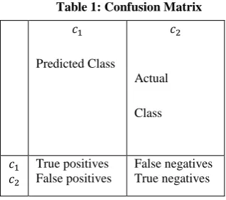
The Confusion Matrix is a useful tool for analyzing how well your classifier can recognize tuples of different classes. A confusion matrix for two classes is shown in Table 1.
[image:3.595.76.235.601.741.2]Given m classes, a confusion matrix is a table of at least size m by m. An entry, in the first m rows and m columns indicates the number of tuples of class i that were labeled by the classifier as class j.
Table 1: Confusion Matrix
The sensitivity and specificity measures can be used to calculate accuracy of classifiers. Sensitivity is also referred to as the true positive rate (the proportion of positive tuples that are correctly identified), while Specificity is the true negative rate (that is, the proportion of negative tuples that are correctly identified).
These measures are defined as follows
Sensitivity = Specificity =
Precision = ( ) where t-pos is the number of true positives tuples that were
correctly classified , pos is the number of positive tuples, t-neg is the number of true t-negatives tuples that were correctly classified, neg is the number of negative tuples, and f-pos is the number of false positives tuples that were incorrectly labeled.
It can be shown that accuracy is a function of sensitivity and specificity:
Accuracy = sensitivity + specificity The above stated performance measures are explained as
below –
TP rate: It is the proportion of actual positives which are predicted as positive. The formula is defines as –
TP rate = Where tp stands for true positive and fn stands for false
negative
FP rate: It is the rate of negatives tuples that are incorrectly labeled. The formula is defined as –
FP rate of class ‘yes’ = FP rate of class ‘no’= Where fp stands for false positive and tn stands for true
negative
Precision: It is the proportion of predicted positive which are actual positive. The formula is defined as –
Precision = Recall: It is proportion of actual positives which are predicted
positive. The formula is defined as –
Recall = F-Measure: It is combination of both precision and recall
that’s why it aggregates the above measure. The formula is defined as-
F-measure = Where pr stands for precision and re stands for recall.
ROC area: This gives the percentage of the area cover under ROC curve. The formula is defined as –
ROC area TP rate = * 100 FP rate = * 100
3.2
Error Measures
The error measures used to find out how far off the predicted value is from the actual known value. Loss functions measure the error between and the predicted value . The most common loss functions are [2]:
Predicted Class
Actual
Class
True positives False positives
37 Absolute error: | - |
Squared error: ( ) Based on the above methods, the error rate is the average loss
over the test set.
Mean absolute error: ∑ | | Mean squared error: ∑ ( ) The mean squared error exaggerates the presence of outliers, while the mean absolute error does not. If we take the square root of the mean squared error, the resulting error measure is called the Root Mean Squared Error.
The formula is defined as – Relative absolute error: ∑∑ | | ̅ | |
Relative squared error: ∑∑ ( ( ̅))
Where ̅ is the mean value of the of the training data, ̅ =
∑
4. WEB DATA
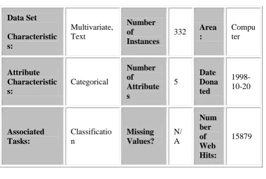
The Web data used in this analysis task is the syskill and webert [10] data which we take from UCI repository. It has a total of 1660 data and a dimension of 332 rows and 5 columns. Only 75% of the overall data is used for training and the rest is used for testing the accuracy of the classification of the selected classification methods. Dataset Description is shown in table 2.
Syskill and Webert Web Page Ratings
4.1
Abstract -
This dataset contains the source of HTML web pages along with them the ratings of a single user on these web pages. The web pages are on four separate subjects (Bands- recording artists; Goats; Sheep; and BioMedical) [11] [image:4.595.47.308.526.701.2]4.2
Data Type
-
html web pages with user ratingsTable 2: Dataset Description
5. WEKA
WEKA is a data mining system developed by the University of Waikato in New Zealand that implements data mining algorithms using the JAVA language. WEKA is a state of-the-art facility for developing machine learning (ML) techniques and their application to real-world data mining problems. It is
a collection of machine learning algorithms for data mining tasks. The algorithms are applied directly to a dataset. WEKA implements algorithms for data preprocessing, classification, regression, clustering and association rules; it also includes visualization tools. The new machine learning schemes or algorithm can also be developed with this package.
WEKA is open source software issued under General Public License [12]. The data file normally used by Weka is in
ARFF file format, which consists of special tags to indicate different things in the data file (foremost: attribute names, attribute types, and attribute values and the data). The main interface in Weka is the Explorer. It has a set of panels, each of which can be used to perform a certain task. Once a dataset has been loaded, one of the other panels in the Explorer can be used to perform further analysis.
Advantages of Weka [13] include:
free availability under the GNU General Public License
portability, since it is fully implemented in the Java programming language and thus runs on almost any modern computing platform
a comprehensive collection of data preprocessing and modeling techniques
ease of use due to its graphical user interfaces Weka's main user interface is the Explorer [13], but essentially the same functionality can be accessed through the component-based Knowledge Flow interface and from the command line. There is also the Experimenter, which allows the systematic comparison of the predictive performance of Weka's machine learning algorithms on a collection of datasets.
The Explorer interface [13] features several panels providing access to the main components of the workbench:
The Preprocess panel has facilities for importing data from a database, a CSV file, etc., and for preprocessing this data using a so-called filtering algorithm. These filters can be used to transform the data (e.g., turning numeric attributes into discrete ones) and make it possible to delete instances and attributes according to specific criteria.
The Classify panel enables the user to apply classification and regression algorithms (indiscriminately called classifiers in Weka) to the resulting dataset, to estimate the accuracy of the resulting predictive model, and to visualize erroneous predictions, ROC curves, etc., or the model itself (if the model is amenable to visualization like, e.g., a decision tree).
The Associate panel provides access to association rule learners that attempt to identify all important interrelationships between attributes in the data. The Cluster panel gives access to the clustering
techniques in Weka, e.g., the simple k-means algorithm. There is also an implementation of the expectation maximization algorithm for learning a mixture of normal distributions.
The Select attributes panel provides algorithms for identifying the most predictive attributes in a dataset.
The Visualize panel shows a scatter plot matrix, where individual scatter plots can be selected and enlarged, and analyzed further using various selection operators.
Data Set
Characteristic s:
Multivariate, Text
Number of Instances
332 Area :
Compu ter
Attribute Characteristic s:
Categorical
Number of Attribute s
5
Date Dona ted
1998-10-20
Associated Tasks:
Classificatio n
Missing Values?
N/ A
Num ber of Web Hits:
6. RESULT
To measure and study the performance on the selected classification algorithms namely Bayes Network Classifier, SMO Function classifier, J4.8 Decision Tree, OneR, ZeroR and Part Rule Learner, we use the same experiment procedure as suggested by WEKA. The 75% data is used for training and the remaining is for testing purposes. In WEKA, all data is considered as instances and features in the data are known as attributes. The simulation results are divided into several sub items for easier analysis and evaluation.
On the first part, correctly and incorrectly classified Instances will be partitioned in numeric and percentage value and Kappa statistic. In the next part, mean absolute error, root mean squared error, relative absolute error and root relative squared error will be consider as parameters for evaluation. The results of the simulation are shown in Tables 1 and 2 below. Table 1 mainly summarizes the result based on accuracy and time taken for each simulation. Table 2 shows the result based on error during the simulation. Figures are the graphical representations of the simulation result.
Table3: Simulation result of bands dataset
Algorithm (Total Instances ,61)
Correctl y Classifie d Instance s % (value)
Incorrectl y Classified Instances % (value)
Time Take n (seco nds)
Kappa Statistic s
J48 96.7213 3.2787 0.02 0.9374
Navies Bayes 93.44261 6.5574 0 0.8759
SMO 85.2459 14.7541 0.03 0.6863
OneR 100 0 0 0.9225
ZeroR 63.93441 36.0656 0.02 0
Part 96.7213 3.2787 0.04 0.9374
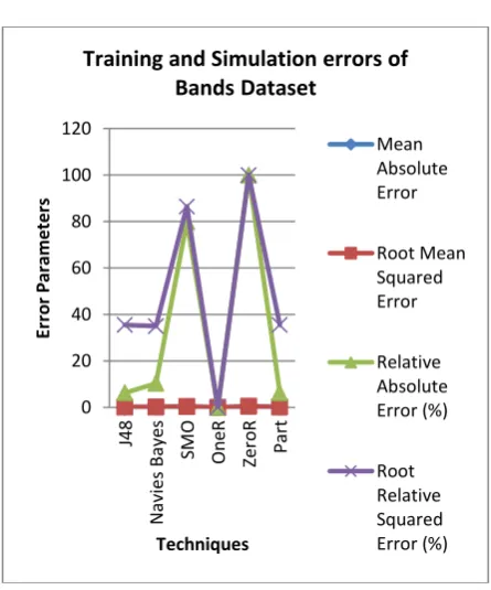
Table 4: Training and simulation result of bands dataset
Algorithm (Total Instances ,61)
Mean Absolute Error
Root Mean Squared Error
Relative Absolute Error (%)
Root Relative Squared Error (%)
J48 0.0219 0.1478 6.2236 35.4681
Navies
Bayes 0.0363 0.1456 10.3275 34.9417 SMO 0.2805 0.3605 79.8701 86.4756
OneR 0 0 0 0
ZeroR 0.3512 0.4168 100 100
[image:5.595.317.540.368.636.2]Part 0.0219 0.1478 6.2236 35.4681
[image:5.595.45.283.510.677.2]Figure 2: Simulation result of bands dataset
Figure 3: Training and simulation result of bands dataset 0
10 20 30 40 50 60 70 80 90 100
J48
N
avie
s B
aye
s
SM
O
O
n
eR
Ze
ro
R
Pa
rt
Par
ame
te
rs
Techniques
Simulation result for Bands Dataset
Correctly Classified Instances % (value)
Incorrectly Classified Instances % (value)
Time Taken (seconds)
Kappa Statistics
0 20 40 60 80 100 120
J48
N
avie
s B
aye
s
SM
O
O
n
eR
Ze
ro
R
Pa
rt
Er
ro
r
Par
ame
te
rs
Techniques
Training and Simulation errors of
Bands Dataset
Mean Absolute Error
Root Mean Squared Error
Relative Absolute Error (%)
39 Figure 4: Simulation Result of TP Rate Parameter
Figure 5: Simulation Result for Bands Dataset
7. DISCUSSION
Based on the above Figures and Tables, we can clearly see that for the Bands Dataset highest accuracy is 100% and the lowest is 63.93%. The other algorithm yields an average accuracy of around 85%. In fact, the highest accuracy belongs to the OneR classifier, followed by J4.8 Decision tree and Part Classifier with a percentage of 96.72% and subsequently Bayes Network Classifier and Sequential minimal Optimization Classifier. ZeroR Classifier present at the bottom of the chart with percentage around 63.93%. An average of 55 instances out of total 61 instances is found to be correctly classified with highest score of 61 instances compared to 39 instances, which is the lowest score. The total time required to build the model is
also a fundamental parameter in comparing the classification algorithm. In this simple experiment, from Table 1, we can say that OneR algorithm requires the shortest time which is around 0 seconds compared to the others. Part algorithm requires the longest model building time which is around 0.04 seconds. The second on the list is J4.8 Decision tree with 0.02 seconds. Kappa statistic is used to assess the accuracy of any particular measuring cases, it is usual to distinguish between the reliability of the data collected and their validity [14]. The average Kappa score from the selected algorithm is around 0.6-0.9. Based on the Kappa Statistic criteria, the accuracy of this classification purposes is substantial [14]. From Figure 2, we can observe the differences of errors resultant from the training of the five selected algorithms. This experiment implies a very commonly used indicator which is mean of absolute errors and root mean squared errors. Alternatively, the relative errors are also used. It is discovered that the highest error is found in ZeroR Classifier with an average score of around 0.5 where the rest of the algorithm ranging averagely around 0.1-0.2. An algorithm which has a lower error rate will be preferred as it has more powerful classification capability, so after analysis we can say that ZeroR algorithm is not suitable for any type of Web Data because it has maximum number of errors and can’t classify the data correctly. OneR is the best technique to classify the Bands and Sheeps dataset where as Navies Bayes is the best option for the classification of biomedical dataset and J4.8 and Part giving their best results for the classification of Goats dataset.
8. CONCLUSIONS
As a conclusion as shown in table 5, we have met our goal which is to evaluate and investigate five selected classification algorithms based on Weka. The conclusion derived from Simulation based analysis as shown in fig 2 is that OneR technique is the best option for classification of bands and sheeps dataset whereas Navies Bayes technique is the best option for biomedical and goats dataset because they correctly classify the instances. This result is given after analysis on highly correctly classified, highly incorrectly classified instances and kappa statistics. Conclusion derived from Training and Simulation errors based analysis as shown in fig 3 is present here. On analysis of various error parameters like RMS error, mean absolute error and root relative error etc. we conclude that OneR method is the best option for classification of band and sheep dataset, Navies Bayes technique is the best option for classification of biomedical, goat and sheep datasets because it has least errors. On the other hand, ZeroR technique is not a good option for classification of any datasets because it has lots of errors. Conclusion derived Dataset based analysis as shown in fig 5 is that OneR is best technique for bands and sheeps dataset and Navies Bayes is a good classification technique for biomedical dataset. In all the datasets, J48 and part are having same result for all the parameters. But J48 and Part techniques are giving their best result for Goats dataset. Whereas ZeroR is a not a good option for classification of all the datasets just because of its highest value for FP rate parameter and lowest value for all the other parameters. After analysis of Technique based analysis, we analyze that OneR is best option for classification of bands and sheeps dataset. Navies Bayes, J48, Part and SMO give their best result for biomedical dataset. But after overall analysis Navies Bayes is a good choice to classify the biomedical dataset among all the other techniques. J48 and Part technique is a good choice to classify the goat dataset. After analysis of Parameter based analysis as shown in fig 4, we can conclude that OneR is a best option for Bands
0.5
0.6
0.7
0.8
0.9
1
1.1
Da
ta
se
ts
Techniques
Simulation Result of TP Rate Parameter
Bands Biomedical Goats Sheeps
0 20 40 60 80 100
J48
N
av
ie
s
B
ay
e
s
SM
O
On
eR
Ze
ro
R
Pa
rt
Pa
ra
m
ete
s
Techniques
Simulation Result for Bands Dataset
Correctly Classified Instances % (value) Incorrectly Classified Instances % (value) Time Taken (seconds)
[image:6.595.57.293.351.580.2]and sheeps dataset. Navies Bayes is a best option for biomedical dataset. J48 and Part techniques are best option for classification of Goats dataset. F-Measure is the only parameter which summarizes all the other parameters and giving best result for all the datasets. So, we can say that F-Measure is the only parameter through which we can accurately classify the given datasets.
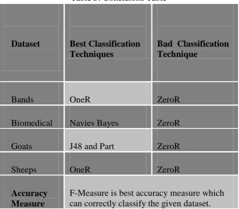
Table 5: Conclusion Table
These results suggest that among the machine learning algorithm tested, OneR and Bayes network classifier has the potential to significantly improve the conventional classification methods that are used to find highly visited web page and lowest visited web pages.
9. REFERENCES
[1] Classification at
http://chem-eng.utoronto.ca/~datamining/dmc/classification.htm [2] Jiawei Han and Micheline Kamber: Data Mining
Concepts and Techniques, Elsevier Inc., Edition 2, 2006, ISBN no. 978-81-312-0535-8
[3] Decision Tree at
http://chem-eng.utoronto.ca/~datamining/dmc/decision_tree.htm [4] Daniel Grossman and Pedro Domingos (2004). Learning
Bayesian Network Classifiers by Maximizing Conditional Likelihood.
[5] Navies Bayes at
http://chem-eng.utoronto.ca/~datamining/dmc/naive_bayesian.htm [6] http://en.wikipedia.org/wiki/Sequential_Minimal_Optimi
zation
[7] http://chem-eng.utoronto.ca/~datamining/dmc/zeror.htm [8] http://chem-eng.utoronto.ca/~datamining/dmc/oner.htm [9] Data Mining Practical Machine Learning Tools and
techniques , Author lan H. Witten & Eibe frank [Part at page number 404 , chapter explorer]
[10]Dataset at
http://archive.ics.uci.edu/ml/datasets/Syskill+and+Weber t+Web+Page+Ratings
[11]http://archive.ics.uci.edu/ml/databases/SyskillWebert/Sys killWebert.data.html
[12]WEKA at http://www.cs.waikato.ac.nz/~ml/weka. [13]http://en.wikipedia.org/wiki/Weka_%28machine_learnin
g%29
[14]Kappa at
http://www.dmi.columbia.edu/homepages/chuangj/kappa [15]Umara Noor , Zahid Rashid, Azhar Rauf: A Survey of Deep Web Classification Techniques. Center of Information Technology, Institute of Management Sciences, Pakistan
[16]Gabriel Fiol-Roig, Margaret Miró-Julià, Eduardo Herraiz : Data Mining Techniques for Web Page Classification. Math and Computer Science Department, University de les Illes Balears , SPAIN {[email protected], [email protected]}
[17]A.Jebaraj Ratnakumar : An Implementation of Web Personalization using Web Mining Techniques. Professor and Head, Department of Computer Science and Engineering, Apollo Engineering College, Chennai, Tamil Nadu, India E-Mail: [email protected] [18]Magdalini Eirinaki, Michalis Vazirgiannis: Web Mining
for Web Personalization. Department of Informatics Athens, University of Economics and Business {[email protected], [email protected]}
[19]Dimitrios Pierrakos, Georgios Paliouras , Charistos Papatheodorou and Constantine D. Spyropoulos: Web Usage Mining as a Tool for Personalization. The Institute of Informatics and Telecommunications, NCSR , email : [email protected]
Dataset Best Classification Techniques
Bad Classification Technique
Bands OneR ZeroR
Biomedical Navies Bayes ZeroR
Goats J48 and Part ZeroR
Sheeps OneR ZeroR
Accuracy Measure