Munich Personal RePEc Archive
Infrastructure and Development
Interlinkage in West Bengal: A VAR
Analysis
Majumder, Rajarshi and Mukherjee, Dipa
2005
Infrastructure and Development Interlinkage in West Bengal: A VAR Analysis
Rajarshi Majumder
Lecturer, Dept. of Economics University of Burdwan, Golapbag
Burdwan, West Bengal - 713104
e-mail: [email protected]
and
Dipa Mukherjee
Lecturer, Dept. of Economics Narasinha Dutt College Belilious Road, Howrah
West Bengal - 711101
Abstract
Theoretical propositions proclaim that the association between Infrastructure Availability and Development of a region is quite strong and runs from the former to the latter. Empirical studies are however, inconclusive. While few researchers have concluded that the impact of infrastructure on development levels, though positive, is not significant, equally large numbers of studies claim that infrastructure explains a substantial part of development levels. In this paper the association between infrastructural availability and development for the West Bengal economy is explored using a multidimensional approach and a time series study. It is observed that both developmental and infrastructural indices have shown a continuously rising trend during 1971-2001. The causation seems to be stronger from infrastructure to development. The long run relationships suggest strong positive impact of infrastructural availability on development levels. Different facets of infrastructure seem to have different impacts on different dimensions of development. A segmented policy aiming at specific sectors need to be adopted, with the greatest importance being attached to those infrastructural indicators that have highest total impact and strongest ‘linkages’ across sectors. Only this can sustain the development ‘push’ generated in West Bengal. Otherwise, the superstructure will have only a weak base and will come crashing down any day.
Infrastructure and Development Interlinkage in West Bengal: A VAR Analysis
Introduction
The association between Infrastructure Availability and Development of a region is a widely discussed and accepted issue. There are a large number of theoretical propositions that conclude that the association is quite strong and runs from the former to the latter [e.g. Hirschman (1958), Rostow (1960), Nurkse (1953), Rosenstein-Rodan (1943) and Hansen (1965)]. Substantial volumes of empirical studies have tried to measure the magnitude of this association, and therein the debate starts. Few researchers have concluded that the impact of infrastructure (or Public Goods) on development levels, though positive, is not significant [e.g. Hulten (1984), Evans (1994), Holtz-Eakin (1994), Crihfield (1995), Conrad (1997)]. On the other side, there are also equally large numbers of studies that claim that infrastructure explains a substantial part of development levels. This second argument seems to have gained wind in the last decade, especially after the publication of the World Bank World Development Report 1994 focusing on Infrastructure. It is now felt that adequate and quality infrastructure is a prerequisite of growth and development. Most of the empirical studies have however concentrated on Cross-sectional studies, wherein regional variation in development and growth were sought to be explained by regional diversity in infrastructural levels. But cross-sectional regions are widely different in socio-economic and technical characteristics. This approach thus includes impact of secular differences in the characteristics of the regions within the impact of infrastructure and tends to overestimate the latter. Secondly, most of these studies use a unidimensional approach with development level being captured by Income or Consumption levels. We try to eliminate these two drawbacks while examining the issue. In this paper we try to explore the association between infrastructural availability and development using a multidimensional approach and for the economy of West Bengal. Thus, a time series study analysing the interaction between infrastructural availability and development levels in West Bengal for the period 1971-2001 is attempted at.
Methodology
Construction of Composite Indices
The multidimensional facets of development is sought to be captured by three broad components - Agricultural development (henceforth Agdev), Industrial development (Inddev) and Human development (Hudev). Similarly, Infrastructural availability is composed of Rural & Agro-specific (Aginf), Transport (Trinf), Power (Powinf), Financial (Fininf), and Social Infrastructure (Socinf). Each of these indicators is composed of more than one indicator and is constructed using the
Modified Principal Component Analysis method from them.1
Agdev is prepared from Land Productivity [Value Added (VA) per hectare Gross Cropped Area (GCA)], Labour Productivity (VA per agricultural labourer), Extent of Commercialisation (% of GCA under commercial crops), and Cropping Intensity (GCA/Net Sown Area). Similarly, Inddev is constructed from Registered Factories per 1000 sq. km. area, % of Net State Domestic Product (NSDP) from manufacturing sector, VA per labour in registered factories, Per capita NSDP from secondary sector, and Factory workers as % of total population. Hudev is prepared from Infant Mortality Rate, Crude Death Rate, Crude Birth Rate (all suitably transformed to reflect positive aspects), Per Capita NSDP (PCNSDP) and Enrolment Ratio in Primary schools. In the second stage, these indices are combined again to yield a single composite index of development (Devt). The standard measure of development – PCNSDP – is also considered separately.
Constituent variables of Aginf are Irrigation Intensity (Net Irrigated Area/NSA), Fertiliser consumption per hectare GCA, Power consumed for agricultural purpose, and Bank Credit to agriculture per hectare GCA. Trinf is composed of Road and Railway length per 1000 sq. km. area, and % of roads surfaced. Powinf consists of % of villages electrified, per capita power generation, and Plant Load Factor (generation as % of generating capacity). Fininf is composed of Bank Branches per 1000 sq. km. Area and per lakh population, Bank credit to Industries per industrial worker, and per capita State Financial Corporation credit off-take. Socinf consists of Hospitals and dispensaries, primary schools, higher educational institutions (all per 1000 sq. km. area), Medical personnel as % of population and State per capita expenditure on primary education.
At the second stage, Aginf, Trinf, and Powinf are combined to yield index of Physical infrastructure (Phyinf). At the third stage, all five first order indices of infrastructure are combined to form a single composite index of infrastructural development (Infra). This method thus provides us 5 Developmental indicators (including PCNSDP) and 7 Infrastructural indicators (Phyinf, Infra, and five sectoral ones) for West Bengal for each of the 30 years from 1971 to 2001. The data have been collected from various sources mentioned in the endnotes.
variability in the constituent variables in all the cases. They are thus reasonably good representatives of the aspects we are looking into. Subsequent analysis is based on these indicators.
Also, this time-series study gives us an opportunity to test whether any structural break in the two series occurred at the initiation of three important changes in policy-regime in West Bengal - the ascension of Left Front to power, and the liberalisation of the economy both at 1984 and at 1991. For these, 1978, 1984 and 1991 are taken as the watershed years and the Dummy Variable technique is used to test for structural breaks at these points of time in the relationship between infrastructural availability and development in West Bengal.
Time Series Study of the Indices
The study of time series requires certain caution while using simple correlation and regression in analysing association and causation between variables. Variables over time, more often than not, have time trends making them non-stationary, and the resultant correlation and regression become spurious. To avoid this, various techniques have evolved over the years. One of them is using the Unit Root Test, the Autocorrelation Function and the Partial Autocorrelation Function to determine the Order of Integration of the different series and then using Engel-Granger (Engel and Granger,
1987) methodology for checking whether the series are co-integrated or not.2 If they are, then OLS can be used. Other methods follow the Box-Jenkins methodology of model selection, testing for causality, identifying dependent and independent variables, and specifying the functional form. If no such clear demarcation is possible, the Vector Auto Regression (VAR) technique is used, which is essentially a Simultaneous system approach. We follow the above path in sequence to explore the relationship between infrastructure and development in West Bengal over the period 1971-2001.
Trends in Infrastructure and Development
Empirical Trends
development, Transport infrastructure, and Financial Infrastructure. Socinf on the other hand has increased till 1986, decreased continuously during 1986-95, and again increased thereafter.
However, we are more interested in the secular (statistical) trends, if any, in the indices and the long run relationship between the infrastructural and the developmental indices.
Statistical Trends in the Indices
To determine the trends in the indices, it has to be tested whether they are Stationary or not. The usual stationarity test, viz. the Augmented Dickey Fuller Test for Unit Root reveals that all the indices are Non-Stationary with one unit root, i.e. they are integrated of order 1. In addition, they also have secular deterministic trend, making them a Mixed Process. The only exception is Fininf, which does not have Unit root but has a trend, making it a Trend Stationary Process.
In addition, the ACF and PACF indicate that the processes also include Autoregressive Error terms of order 1 in all the indices. Only for Socinf, an AR(3) process is indicated.
We also tried to examine whether there has been any structural breaks in the trends shown by the indices during the three time-points – 1978, 1984, 1991. Presence of no such structural breaks could be detected in any of the indices.
Direction of Causality
Considering that the indices are non-stationary, simple OLS method of estimating the relationship between them is ruled out, at least for the time being. Also, it has to be accepted that there may be bi-directional causation between infrastructural and developmental indices. Consequently, the System method should be preferred for estimation. Each of the five developmental indices paired with each of the seven infrastructural indices yield 35 possible systems. These systems are estimated using Vector Auto Regression (VAR) technique. The length of the lags to be included in each system is determined in a trial and error method using the usual information criteria like Akaike Information Criterion (AIC), Schwartz Criterion (SC) and Likelihood Ratio (LR). Once the lengths of the lags are decided, the systems are tested for Causality using Granger causality test.
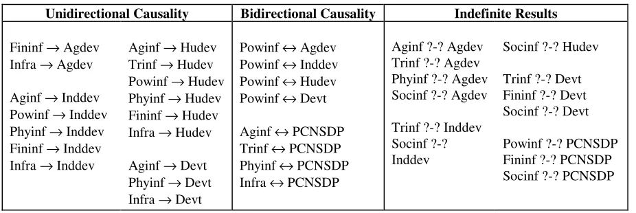
It is observed that the results indicate strong unidirectional causality in most of the systems involving Inddev, Hudev and Devt, where the causation runs from Infrastructure to Development (Table 1). However, for PCNSDP, bi-directional causality seems to operate between the infrastructural indices and PCNSDP. This is true for Powinf also, where there seems to be bi-directional causality between the developmental indices and Powinf. For the other systems, especially for those involving Agdev, no strong causality is hinted at by the Granger tests, thereby making the conclusions indecisive. This vindicates our use of System method. The solution of the VAR models however, provides further insight into the causality.
shocks in developmental indices. Moreover, the responses in the former case are found to be increasing in subsequent periods, while in the later case they are found to be decreasing with time. Variance Decomposition reveals that substantial portion of variation in developmental indices can be attributed to variance in infrastructural indices. On the contrary, the proportion of variation in infrastructure attributable to development indices is quite low. It has to be noted that these results depend crucially on which variable (developmental or infrastructural) is mentioned first in the order of model-solve in the computational programme. So the models were solved by reversing the order also (i.e. mentioning infrastructural indices first). It comes out that in such cases the patterns of the results are similar to the earlier one, though the magnitude of impulse responses or variance decomposition are much lower than before. Thus, it can be reasonably argued that though there is bi-directional causality between infrastructural and developmental indices, the causation is stronger from infrastructure to development rather than the other way round. It is development that seems to depend on infrastructural availability.
Long Run Relationship
Once the matter of causation is decided, we turn towards the long run relationship (LRR) between the indices. As such, the main objective of this study is to estimate the LRR between the developmental and infrastructural indices in West Bengal and deduce the implications thereof.
The VAR technique gives us an approximation of the functional relationship between the indices. However, these are unrestricted regressions and one possibility regarding regression between integrated and non-stationary series is that of Cointegration. If two series are cointegrated, then the LRR between them can be approximated by the Cointegrating Equation (CE). And if two series are cointegrated, then the vector regression has to be restricted by this LRR and has to be solved by Vector Error Correction (VEC) technique, rather than VAR.
The Johanssen Multi-equation test for Cointegration is used here. Inclusion of intercept and/or trend in the CE is decided by the usual information criteria (minimum AIC and SC, and higher Likelihood Ratio). Once the suitable model is specified, the tests for presence of CE are performed. It is observed that of the 35 systems, in 17 cases presence of CE is not indicated. For these systems that do not indicate presence of cointegration, the VAR results are retained. For the other 18 cases where presence of CE is indicated, the CE is taken to be the LRR between the two variables. Once presence of a CE is confirmed, we solve the vector model using VEC. The solution of VEC is not used as the LRR though. The coefficient of the CE in the VEC model would determine whether the LRR is stable or not. If the coefficient of CE in the equation, where the LHS variable is that one which is the first one (or the normalised one) in the CE, is negative, we can say that the LRR is stable. To be more
elucidating, let the CE be x1t - α - β x2t, and the VEC be ∆x1t = ∆x2t + θ [x1t-1 - α - β x2t-1]. Let in
be relatively more (less) than ∆x2 and they will diverge further. If on the other hand, θ is negative,
then ∆x1 will be relatively lower (greater) than ∆x2 and the gap between them will decrease and the
LRR will be restored. And once LRR is achieved, i.e. the CE becomes valid, for the subsequent
periods ∆x1 will be equal to ∆x2 and the equilibrium will continue.
It is evident from the results that of the 18 CE-s obtained, for 16 systems the CE-s are stable and provide the LRR between the developmental and infrastructural indices. Only 2 relations – that of PCNSDP with Trinf and Socinf - is observed to be unstable. This result may be due to wrong specification of the Cointegrating model. Other model specifications should be used to find out if any Stable LRR for this system is yielded. This issue has not been probed further.
The final estimated models in terms of the coefficients of infrastructural indices with developmental indices as dependent variables are reported in Table 2.
Another parameter of interest in case of the VEC models is the Speed of Adjustment or the coefficient of the Error Correction term or CE. As has been reported earlier, of the 18 VEC models, the CE yields stable relation in 17 cases. The speed of adjustment parameters for these are reported in Table 3. It is observed that the effect of any short-run discrepancy between the actual and long run equilibrium values of the variables is quite substantial and the speeds of adjustment are quite substantial in many cases.
Final Estimated Models
It is observed from the estimated models that the coefficients of the infrastructural indices are almost always positive (Table 2). In most of the cases they are significant also. This indicates that changes in infrastructural indices would lead to significant impact on developmental levels in the subsequent periods. Considering that many of the estimated results are long run relations, the stability of the estimated models should also be quite robust. In fact, as mentioned earlier, Dummy Variable Technique has also been used to test for structural breaks in the relationships at important historical datelines like 1978, 1984 and 1991. In none of the cases any significant structural break can be traced. Consequently, it can be reasonably argued that the model estimates depict the relationship between developmental and infrastructural indices for West Bengal.
An Extension – The Multivariate Situation
Fininf are positive, while that of Socinf is insignificant but negative (Table 4). On removing Socinf, the VAR system gives a better fit, and the coefficients are significant. Similar results are obtained with Inddev and Devt, where removal of Socinf gives a better fit. It seems that since Socinf has been following AR(3) process while the others are following AR(1) process, inclusion of Socinf affects the specification of the model. For Hudev however, presence of CE is not confirmed and we persist with Multivariate VAR. The results of the Multivariate exploration are summarised in Table 4. Most of the coefficients are significantly positive. The speed of adjustment is also significant in all three cases. It therefore follows that the infrastructural indices taken together affects the developmental indices significantly, and any short run inconsistency is speedily corrected. This again underlines the importance of a comprehensive infrastructural development programme for development of the state.
Summary Results and Impact of Individual Infrastructural Factors
The main features of the estimation results may be discussed further. The Long Run Multipliers can be obtained by adding up the Impact Multipliers or the coefficients of the lagged terms of the variables, for the VAR models. For the VEC models the multipliers are directly obtained from the CE.
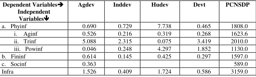
It is observed that for agricultural & industrial developmental indices and for PCNSDP, the highest multiplier is associated with Transport infrastructure, indicating its prime importance in shaping the development profile of the region (Table 5). Multipliers of Physical infrastructure are greater than those of Financial or Social infrastructure. It thus follows that the authorities should attach adequate importance to development of physical infrastructure, especially those related to transport and power, to augment development levels in West Bengal. Agricultural infrastructure has generally low multiplier except for PCNSDP, where it has the second largest multiplier. If we now look at the magnitude of individual impacts, we find that improvements in Transport infrastructure leads to more than proportionate improvement in Agricultural and Industrial development, and the composite development index Devt (the multipliers being greater than unity). The impact of the composite index of infrastructure (Infra) is observed to be highest for Human development, indicating the importance of infrastructural expansion for even the ‘non-economic’ dimension of development.
agricultural development will be better augmented by improvements in financial facilities rather than by conventional agricultural infrastructural facilities.
Conclusion and Policy Implications
The conclusions that can be drawn may be summarised as -
• Both developmental and infrastructural indices have shown a continuously rising trend
during 1971-1995. Only Social infrastructure has shown an inverted U-shaped pattern.
• The Causation seems to be stronger from infrastructure to development, though in some
cases bi-directional causality cannot be ignored.
• The long run relationships suggest strong positive impact of infrastructural availability on
development levels.
• Differential impact of the various infrastructural sectors on sectoral and overall
development level has been underlined.
The policy suggestions that emerge from this study can be briefly mentioned. It is quite obvious that infrastructural expansion is a necessary condition for development of the West Bengal economy. Moreover, different facets of infrastructure have different impacts on different dimensions of development. A segmented policy aiming at specific sectors need to be adopted with the greatest importance being attached to those infrastructural indicators that have highest total impact across agricultural, industrial and human development. For example, in our study, Transport and Power sectors emerge as most significant policy instruments having the strongest ‘linkages’. Given the poor condition of the roads, inadequate rural connectivity, low per capita power consumption and low PLF in the state, there are long strides to be taken in those areas. These would naturally lead to substantial improvement in the development levels in all the segments. However, further analysis using a multivariable VAR/VEC method or a comprehensive macroeconomic modelling should be attempted before these ideas can be given definite shape. This is one possible extension of the study. In addition, the relationships may be used to simulate and forecast the path of developmental indices under different assumptions regarding infrastructural expansion.
The bottom-line is that infrastructure has been playing a crucial role in shaping the development profile of West Bengal and this sector has to be carefully nurtured to reap the benefits of a stable administration and some sort of rural land redistribution that has already occurred here. Otherwise, the superstructure will have only a weak base and will come crashing down any day.
___________________________
Notes
1
The modified PCA method, MODPCA, has been evolved by Amitabh Kundu and Moonis Raza. Refer to Kundu and Raza (1982).
2
Table 1
Direction of Causality - according to Granger Causality test
Unidirectional Causality Bidirectional Causality Indefinite Results
Fininf → Agdev Infra → Agdev Aginf → Inddev Powinf → Inddev Phyinf → Inddev Fininf → Inddev Infra → Inddev
Aginf → Hudev Trinf → Hudev Powinf → Hudev Phyinf → Hudev Fininf → Hudev Infra → Hudev Aginf → Devt Phyinf → Devt Infra → Devt
Powinf ↔ Agdev Powinf ↔ Inddev Powinf ↔ Hudev Powinf ↔ Devt Aginf ↔ PCNSDP Trinf ↔ PCNSDP Phyinf ↔ PCNSDP Infra ↔ PCNSDP
Aginf ?-? Agdev Trinf ?-? Agdev Phyinf ?-? Agdev Socinf ?-? Agdev Trinf ?-? Inddev Socinf ?-? Inddev
Socinf ?-? Hudev Trinf ?-? Devt Fininf ?-? Devt Socinf ?-? Devt Powinf ?-? PCNSDP Fininf ?-? PCNSDP Socinf ?-? PCNSDP
Table 2
Final Estimated Models – Developmental Indices regressed on Infrastructural Indices Dependent Variables
Independent Variables✁✁
Agdev Inddev Hudev Devt PCNSDP
Constant 1.257** 1.832** 1.859** 1.235** 729.6* Trend
Aginf 1623.6
Aginf(t-1) 0.526** 0.216** 0.319** 0.268**
Model Specification VAR VAR VAR VAR CE/LRR Constant -1.267* 0.639** 1.692** 0.537*
Trend
Trinf 3.419** 2010.0** Trinf(t-1) 2.703** 0.882* 0.075**
Trinf(t-2) 2.186** 1.429** Trinf(t-3) 0.199 0.004
Model Specification VAR VAR VAR CE/LRR CE/LRR Constant 1.163** 1.586** 2.194* 269.0 Trend 0.066** 0.015 0.174
Powinf 4.297** 1.852*
Powinf(t-1) 0.046 0.248* 1130.0**
Model Specification VAR VAR CE/LRR CE/LRR VAR
Constant 0.880
Trend 0.003
Phyinf 0.690* 0.729** 7.738 0.465** 1808.0** Phyinf(t-1)
Model Specification CE/LRR CE/LRR CE/LRR CE/LRR CE/LRR Constant 1.612* 2.491 1.632** 1.474*
Trend -65.0*
Fininf 0.614** 0.145* 0.297**
Fininf(t-1) 0.425** 1597.0**
Model Specification CE/LRR CE/LRR VAR CE/LRR VAR Constant 1.373
Trend
Socinf 589.0*
Socinf(t-1) 0.363 Socinf(t-2)
Model Specification VAR VAR VAR VAR CE/LRR Constant 1.344
Trend
Infra 1.526** 1.724** 0.586* 3159.0** Infra(t-1) 0.409**
Model Specification CE/LRR VAR CE/LRR CE/LRR CE/LRR VAR – model estimated by VAR; CE/LRR – models from the Cointegrating equation; * and ** refers to significance at 5% & 1% levels respectively. Coefficients with significance level more than 10% are not reported.
Table 3
Speed of Adjustment in Error Correction Models – Coefficients of Cointegrating Equation Dependent Variables✂✂
Independent Variables✄✄
Agdev Inddev Hudev Devt PCNSDP
Aginf 0.055**
Trinf 0.215* 0.126**
Powinf 0.051 0.022*
Phyinf 0.063** 0.001 0.004 0.854** 0.090** Fininf 0.132** 0.083 0.013 0.126*
Socinf 0.129**
Infra 0.068* 0.009 0.016**
Note: * and ** refers to significance at 5% & 1% levels respectively. Coefficients with significance level more than 10% are not reported.
[image:13.595.78.520.279.515.2]Source: Authors’ calculation.
Table 4
Multivariate Models – Developmental Indices regressed on All Three Infrastructural Indices Dependent
Variables✂✂
Independent Variables✄✄
Agdev Inddev Hudev Devt
Model 1 Model 2 Model 1 Model 2 Model 1 Model 2 Model Specification CE/LRR CE/LRR CE/LRR CE/LRR VAR CE/LRR CE/LRR
Constant 0.223 0.490 0.550
Trend 0.108* 0.016
Phyinf 1.248** 0.958** 1.218** 1.122** 0.405** 0.720** Fininf 0.023 0.183 -0.494* 0.774** 0.134* 0.103 Socinf 0.078 0.348** -0.060
Phyinf(t-1) 0.609** Fininf(t-1) 0.035 Socinf(t-1) 0.556** Socinf(t-2)
Speed of Adjustment
0.033 0.543* 0.129 0.227* 0.588* 0.280*
Note: VAR – model estimated by VAR; CE/LRR – models from the Cointegrating equation; Speed of Adjustment is the Coefficient of the Error Correction Term in VEC Models. * and ** refers to significance at 5% & 1% levels respectively. Coefficients with significance level more than 10% are not reported.
[image:13.595.89.509.628.755.2]Source: Authors’ calculation.
Table 5
Final Multipliers on Developmental Indices for Changes in Infrastructural Indices
Dependent Variables✂✂
Independent Variables✄✄
Agdev Inddev Hudev Devt PCNSDP
Note: Coefficients with significance level more than 10% are not reported and Multipliers are also not reported for them.
[image:14.595.78.521.150.507.2]Source: Authors’ calculation.
Table 6
Impact of Increment in Different Instrumental Variables on Individual Development Indices
Impact on
Impacts of 1 unit increment in Agdev Inddev Hudev Devt PCNSDP
Fertiliser consumption per hectare GCA 0.231 0.095 0.140 0.118 714.4
Irrigation Intensity 0.211 0.087 0.128 0.107 651.1
Bank Credit To Agriculture per hectare GCA 0.252 0.103 0.153 0.128 777.7
Power Consumed by Agricultural sector 0.339 0.139 0.206 0.173 1047.2
Road and Railway length per 1000 sq. km. Area 3.618 1.646 0.053 2.431 1429.1
% of Roads Surfaced 3.577 1.627 0.053 2.404 1413.0
% of Villages electrified 0.028 0.149 2.578 1.111 678.0
Per capita power generation 0.027 0.144 2.488 1.072 654.3
PLF 0.025 0.137 2.372 1.022 623.8
Bank branches per 1000 sq. km. area 0.312 0.074 0.216 0.151 811.3
Bank branches per lakh pop 0.300 0.071 0.207 0.145 779.3
Bank credit to SSI 0.301 0.071 0.208 0.146 782.5
Per Capita SFC credit 0.315 0.074 0.218 0.152 819.3
Primary Schools per 1000 sq. km. Area 0.149 241.5
Secondary Schools per 1000 sq. km. Area 0.149 241.5
Per capita expenditure on Pr. Schools 0.148 240.9
Colleges per 1000 sq. km. Area 0.148 239.7
Hospitals per 1000 sq. km. Area 0.148 239.7
Medical Personnel as % of pop 0.147 239.1
Note: Impacts are obtained by multiplying individual Factor Loadings with the Final Multipliers from Table 3b. Coefficients with significance level more than 10% are not reported and impacts are not assessed for them.
Source: Authors’ calculation.
Data Sources
FAI - All India Fertiliser Statistics, Various Years
GOI - Annual Survey of Industries - Summary Results for Factory Sector, Min. of Statistics and Programme Implementation, Various Years
GOI - Basic Road Statistics, Min. of Surface Transport, Various Years
GOI - Education in India, Dept. of Education, Min. of HRD, Vol. I (s) and II (c), Various Years GOI - Health Statistics in India, Min. of Health and Family Planning, Various Years
GOI - Indian Agricultural Statistics, Ministry of Agriculture, Various Years
GOI - Selected Educational Statistics, Dept. of Education, Min. of HRD, Various Years
RBI - Banking Statistics - Basic Statistical Returns, Various Years
Registrar General of India - Sample Registration System, Min. of Home Affairs, GOI, Various Years
References
Conrad, K. and H. Seitz - Infrastructure Provision and International Market Share Rivalry, Regional Science and Urban Economics, Vol. 27, 1997
Crihfield, J.B. and M.P.H. Panggabean - Is Public Infrastructure Productive? A Metropolitan Perspective Using New Capital Stock Estimates, Regional Science and Urban Economics,
Vol. 25, 1995
Enders, W. - Applied Econometric Time Series, John Willey and Sons, 1995.
Engle, R.F. and C.W.J. Granger - Co-integration and Error Correction: Representation, Estimation, and Testing, Econometrica, Vol. 55, No. 2, 1987.
Evans, Paul and G. Karras - Is Government Capital Productive? Evidence from a Panel of Seven Countries, Journal of Macroeconomics Vol.16, No.2, Spring, 1994
_____________ - Are Government Activities Productive? Evidence from a Panel of US States,
Review of Economic and Statistics Vol.76, No.1, February, 1994
Granger, C.W.J. - Investigating Causal Relations by Econometric Models and Cross-Spectral Methods, Econometrica, July, 1969
Hansen, N. - The Structure and Determinants of Local Public Investment Expenditure, Review of Economics and Statistics (47), 1965
_____________ - Unbalanced Growth and Regional Development, Western Economic Journal,
1965a
Hirschman, A.O. - The Strategy of Economic Development, Yale University Press, New Haven, 1958 Holtz-Eakin, Douglas - Public Sector Capital and Productivity Puzzle, Review of Economics and
Statistics Vol.976, No.1, February, 1994
Hulten, C.R. and G.E. Peterson - The Public Capital Stock: Needs Trends and Performances,
American Economic Review Vol.74, May, 1984
Johansen, Soren - Estimation and Hypothesis Testing of Cointegration Vectors in Gaussian Vector Autoregressive Models, Econometrica, Vol. 59, 1991
Kundu, Amitabh and Moonis Raza - Indian Economy - The Regional Dimension, Spectrum Publishers, New Delhi, 1982
Mills, T.C. - Time Series Techniques for Economists, Cambridge University Press, 1990 Nurkse, R. - Problems of Capital Formation in Underdeveloped Countries, Oxford, 1953
Rosenstein-Rodan, P. - Problems of Industrialisation of Eastern and South-Eastern Europe, The Economic Journal, 1943
Rostow, W.W. - The Stages of Economic Growth A Non Communist Manifesto, Cambridge University Press, 1960
Townsend, R.F. - Econometric Methodology II: Strengthening Time Series Analysis, Agrekon, Vol. 37, No. 1, March, 1998