Munich Personal RePEc Archive
Benefit Transfer: Conceptual Problems
in Estimating Water Quality Benefits
Using Existing Studies
Desvousges, William H. and Naughton, Michael C. and
Parsons, George R.
March 1992
Online at
https://mpra.ub.uni-muenchen.de/45028/
Benefit Transfer: Conceptual Problems in Estimating Water
Quality Benefits Using Existing Studies
WILLIAM DESVOUSGES MICHAEL NAUGHTON
GEORGE PARSONS
University of Delaware
1992
INTRODUCTION
In February 1981, President Reagan signed Executive Order 12291 requiring that all new major regulations be subject to benefit-cost analysis. In keeping with this order,
the U.S. Environmental Protection Agency (EPA) devel- oped guidelines for performing its own benefit-cost analyses (EPA, guidelines for regulatory impact analyses, 1982). Because of limited research budgets and time for preparing such analyses, EPA suggests that "off-the-shelf methodolo- gies and studies can serve as the basis for benefit-cost analysis." That is, where possible, benefits and costs should be inferred from the results of existing research studies.
Prominent examples of this strategy include the proposed water quality regulations in the iron and steel industry [EPA, 1982], the Boston combined sewer overflow systems [Meta Systems, Incorporated, 1985], and the pulp and paper indus- try [Naughton and Desvousges, 1986].
We call the use of existing studies "benefit transfer." The river where an existing study was conducted is termed the "study site" and the river under consideration for water quality improvements the "policy site." The estimated benefits are "transferred" from the study site to the policy site.
Not surprisingly, the low cost and shorter time require- ments make benefit transfer an attractive policy evaluation alternative. The social cost of benefit transfer, however, may come in the form of poor quality benefit estimates that could lead to incorrect policy choices. In depth studies that are tailored to the policy site are likely to reduce the error in benefit estimates. The rub, of course, is that these studies take more time and money than benefit transfer.
This paper assesses the potential usefulness of benefit
transfer in policy evaluation. For illustration, we use an analysis that we conducted for the EPA on the pulp and paper industry. We raise some conceptual issues that we hope will shed some light on the goals of benefit transfer, its present level of accuracy, and its overall role in policy evaluation. We also investigate some of the empirical prob- lems and issues that arise in using benefit transfer. Given the shortcomings encountered in using existing valuation studies for benefit transfer, we conclude by identifying important areas for future research. Specifically, we make recommen- dations for the design of future valuation studies that would contribute to improving the reliability of transfer.
AGENCY EVALUATION DECISIONS AND BENEFIT TRANSFER
Government agencies routinely face difficult regulatory decisions involving water resources. The EPA's recent task of evaluating the benefits of best conventional control tech- nology (BCT) regulations for the pulp and paper industry is probably a typical example. These regulations would reduce biological oxygen demand (BOD) and total suspended solids (TSS) discharges from 21 pulp and paper plants located primarily in the northeast United States. Thus, the EPA was faced with the challenge of estimating the benefits of regu- lations for 21 different river segments within the confines of a 6-month regulatory time frame.
To illustrate the key issues involved in such an evaluation decision, we specify a simplified model of the EPA's deci- sion problem. As shown in (1), the EPA wants to minimize the mean square error (MSE) in its benefit estimates <in for these 21 river segments subject to the evaluation constraints on both the available funds (AF) and the available time (AT) for the evaluation.
Minimize MSE (B) = Var (B)
+
(Bias (B)) 2subject to AF = AF0 and AT
=
AT 0 •(1)
The MSE framework provides a useful conceptual basis for considering the evaluation choices of EPA because it addresses both the bias and variance aspects of benefit estimation. Using Mitchell and Carson's [1989] terminology, the bias component addresses the concept of validity: Are the benefit estimation methods, or benefit transfer ap- proaches, measuring the "true" benefits from the regula- tions? The variance component addresses the related con- cept of reliability: How reliable, or accurate, are the benefit estimation methods?
Our formulation of the decision problem faced by govern- ment agencies explicitly acknowledges that both time and financial resources are limited. For our specific example, the EPA was faced with the task of evaluating benefits at a number of different river segments within a short time frame. This was only one of many water quality evaluation tasks that the agency was facing at the same time, which gives some indication of the usefulness of an evaluation process like benefit transfer.
The use of benefit transfer may in fact be the most appropriate solution to the above constrained optimization problem. However, before this can be determined, critical questions must be answered, such as, how large is the MSE on the benefit estimates and at what point does this error become intolerable for policy evaluation purposes? If the shortcomings of existing valuation studies when used in benefit transfer are too large, then this leaves the agency with three choices. First, the EPA could abandon its current objective function as unrealistic under the current con- straints. Second, the time and money constraints on the objective function could be relaxed, so that original studies could be conducted for at least some of the policy sites. Third, an attempt could be made to improve the applicability of original studies for transfer exercises. We tum now to a closer look at benefit transfer.
A CONCEPTUAL OVERVIEW OF BENEFIT TRANSFER
This section offers a conceptual perspective on the issue of benefit transfer. Its purpose is to illustrate the issues that arise in transfer and to consider how one might address them. Because of data and model limitations, we are unable to derive any testable hypotheses. Nonetheless, our frame- work may provide a basis for such testing if models and data become available.
For purposes of illustration we can think of the goal of benefit transfer as an attempt to construct the best prediction equation possible for estimating the benefits of water quality improvements at policy sites using existing studies. We write a general form of a prediction equation for a given household as
E(csiX) = f(Q 1 - Q0 , a, {3, P; c5). (2)
E( ) is an expected value operator; c5 is a vector of parameters; cs is compensating surplus for an improvement in water quality from Q0 to Q 1 ; a is a vector of household
characteristics such as income and household size; {3 is a vector of site characteristics of the river such as natural cover, size, and recreation accommodations; Pis a vector of own and substitute implicit prices of recreation visits; and X= (Q 1 - Q 0 , a, {3, P).
Assuming the models and data are available, the transfer problem is straightforward. We know the values of Q 1 -
Q0 , a, (3, and P for households at a policy site and need to
predictte
at that Site. To predict the expected compensating surplus1 for households we need estimates of the parameters
a.
Because of limited time and research resources, we must use estimates from existing valuation studies. Typically, these are studies conducted on rivers other than the policy site. In this ideal transfer we would have estimates for each parameter in the vector c5. Using these parameter estimates and the values of (Q 1 - Qo). a, {3, and P for each household at the policy site, the transfer can be conducted in a two-step process. First, we establish the market area. This is the geographic area defined so that the compensating surplus of households at its boundaries is zero. Market size is critical in determining a very important element in the transfer process, which is the population size used to con- vert benefits per household to aggregate benefits. Second we substitute the parameter estimates and variables for each household in the market area into an expression such as (2)and compensating surplus is estimated. The sum of the individual household estimates over the market area is the
estimate of the aggregate market benefits of the improve- ment.
The problem in actually undertaking a transfer is that the quality of the parameter estimates varies across studies and
many studies do not estimate all the necessary parameters. Studies also vary in the components of user, nonuser option. and existence benefits that they attempt to measure. Exist- ence values are very difficult to address in a transfer exer- cise, since few studies are available which attempt to esti- mate them. Further, estimates of water quality changes, household and site characteristics, and implicit prices at the policy site are often poor. All these problems make it difficult to either accurately define the market or to calculate per- household benefits. In an attempt to reduce the difficulties encountered in benefit transfer, we attempted to employ five criteria to select among studies available for transfer.
Our first criterion heeds the advice of Freeman [1984] that to reduce transfer error, it is necessary to have studies that are based on adequate data, sound economic method and
correct empirical technique. In effect, the studies to be transferred must pass scientific muster. An example of an effort to develop guidelines of credibility are the reference operating conditions developed by Cummings et al. [1986] for the appropriate application of contingent valuation meth· ods. These conditions place limits on the relevant circum· stances under which the contingent valuation method should be applied. For example, the contingent valuation method should not be applied to analyze sensitive political issues where there is reason to believe responses will affect imme- diate outcomes.
Our second criterion is that the change in water quality valued at the study site should be similar to the expected change at the policy site. Because the relationship between willingness to pay and water quality is probably nonlinear. we want to avoid extrapolating from study sites with large water quality changes to policy sites with small changes.
[image:4.612.74.545.86.260.2]
TABLE I. Policy Sites
Current Reduction in Qualitative
Loadings,a Current Affected Assessment of
Current mg/L Loadings, a % Reach per-Family
PolicY Site Water Dilution Length,d Benefits Due
River Largest City in Market Area Qualitya BODb TSSb BOD TSS Ratea,c miles to Reduction
Westfield Northhampton, Massachusetts swimmable 13.77 4.49 45 0 9.62 20-25 moderate
Hudson Glen Falls, New York boatable 11.67 6.42 57 0 16.42 25-35 moderate
Schuylkill Philadelphia, Pennsylvania fishable 22.09 2.15 86 0 44.74 5-10 low/moderate
SalmOn Oswego, New York fishable 4.6 1.97 35 0 6.88 10-20 low/moderate
Oswegatchie Canton, New York boatable 4.11 5.35 0 12 3.97 20-30 low/moderate
St. John Presque Isle, Maine fishable 6.6 3.48 55 0 32.28 20-30 low/moderate
Androscoggin Berlin, New Hampshire fishable 3.4 2.72 12 0 48.08 20-25 low/moderate
Umestone Syracuse, New York fishable 10.52 21.24 75 73 5.88 5-10 low
Fox Green Bay, Wisconsin fishable 6.56 11.97 0 22 11.92 20-30 low
Kennebec Augusta, Maine fishable 18.26 30.76 51 59 225.21 10-15 low
Ashuelot Keene, New Hampshire swimmable 10.40 8.33 55 16 42.86 5-10 low
Black Lowville, New York fishable 21.21 28.71 54 46 50.81 20-25 low
I mile equals 1.609 km.
"Source: EPA, Office of Water Regulations and Standards.
bBOD denotes biological oxygen demand; TSS, total suspended solids.
'Dilution rate is the ratio of the river's low flow to the point source (pulp and paper plants) flow.
dne affected reach length is a qualitative assessment based on the current loadings and expected percentage reduction in loadings in consultation with state water quality officials.
'Moderate denotes noticeable water quality improvement which should affect recreational/aesthetic enjoyment. Low denotes minor water quality improvement which may affect recreational/aesthetic enjoyment.
Our fourth criterion is that the study and policy sites be similar. Alternatively, the study site model should contain regression results that describe willingness to pay as a function of site characteristics. Vaughan and Russell
[1982a], Brown and Mendelsohn [1984], Bockstael et al.
[1986], and Smith and Desvousges [1986] all found that site characteristics are important. Study and policy sites should
also have similar populations. Preferences of households may differ not only by socioeconomic grouping, but also by region of the country.
Our fifth criterion is that, short of usable information on own and substitute implicit prices from the study site, the markets for the study site and policy site be similar. Recent work by Brown and Mendelsohn [1984] and Bockstael et al. [1986] suggests that own and substitute prices are important determinants of willingness to pay. Our fifth criterion implic- itly assumes that there is a strong relationship between a site's market and the implicit prices for that site.
A BENEFIT TRANSFER CASE STUDY
The Policy Sites
Our case study involves EPA's decision of whether or not to increase water pollution controls from best practical to best conventional technology for various pulp and paper production processes. The proposed regulations were ex- pected to reduce pollutant loadings on 21 rivers. Nine of these were expected to have no improvement because the reduction in loadings relative to the total flow of the river was minuscule. We assumed zero benefits on these rivers
and applied our transfer to the remaining 12 listed in Table 1. The data presented in Table 1 are on the current water quality and the potential for changes in water quality due to the proposed regulation for each site. Current water quality level is expressed as a qualitative measure that ranges from boatable to drinkable. EPA provided estimates of the ex-
pected reduction in pollutant loadings due the regulation, but no estimates were made for the expected change in water quality. To assess the potential for water quality change, we present measures of current pollutant loadings for biological oxygen demand (BOD) and total suspended solids (TSS), expected reductions in those loadings, and a dilution rate. The dilution rate is defined as the total flow of the river during the near low flow period divided by the average flow from plants on the river. Plant flow includes all discharges, pollutant and nonpollutant, to the river. Lower dilution rates and larger reduction of loadings suggest a higher potential for water quality improvement. The length of the affected reach is also provided and is defined as that portion of the river which should experience water quality improvements as a result of the proposed regulations.
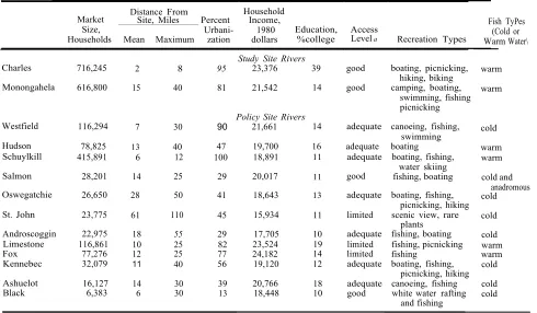
Finally, a qualitative assessment of potential per- household benefits due to the proposed regulations is also presented in Table 1. These assessments will be compared to the quantitative transfer estimates later in this section. These assessments are based both on the expected reduction in pollutant loadings and on a profile of each policy site. These profiles, from Naughton and Desvousges [1986], are sum- marized in Table 2 and include socioeconomic characteris- tics of users and site characteristics of the rivers. The most important site characteristic in determining the qualitative assessments is access. As defined in the footnote to Table 2, access measures how easy it is for users to get to and use the site for recreation and the quality of accommodations for recreations. Sites ranked as moderate have a noticeable potential for water quality improvement and have adequate access. Those ranked as low would have a minor potential for water quality improvement or limited access.
Selection of the Study Sites
pub-Distance From Household
Market Site, Miles Percent Income,
Size, Urbani- 1980 Education, Access
Households Mean Maximum zation dollars %college Level a Recreation Types
Charles 716,245 2 8 95 23,376 39 good boating, picnicking,
hiking, biking warm
Monongahela 616,800 15 40 81 21,542 14 good camping, boating,
swimming, fishing warm
picnicking
Westfield 116,294 7 30 90
Policy Site Rivers
21,661 14 adequate
canoeing, fishing,
cold swimming
Hudson 78,825 13 40 47 19,700 16 adequate boating warm
Schuylkill Salmon 415,891 28,201 6 14 12 25 100 29 18,891 20,017 11 11 adequate good
boating, fishing, water skiing fishing, boating
warm
cold and
Oswegatchie 26,650 28 50 41 18,643 13 adequate boating, fishing, cold
picnicking, hiking
St. John 23,775 61 110 45 15,934 11 limited scenic view, rare cold
plants
Androscoggin 22,975 18 55 29 17,705 10 adequate fishing, boating cold
Limestone 116,861 10 25 82 23,524 19 limited fishing, picnicking warm
Fox 77,276 12 25 77 24,182 14 limited fishing warm
Kennebec 32,079 11 40 56 19,120 12 adequate boating, fishing, cold
picnicking, hiking
Ashuelot 16,127 14 30 39 20,766 18 adequate canoeing, fishing cold
Black 6,383 6 30 13 18,448 10 good white water rafting cold
and fishing
TABLE 2. Study and Policy Site Attributes
Study Site Rivers
Fish TyPes (Cold or Warm Water\ anadromous
1 mile equals 1.609 km.
a Good denotes plenty of easy access sites; adequate, a moderate level of access sites and/or some degree of difficulty in accessing the
river; limited, a few access sites and/or very difficult river access (e.g., steep embankments or no public accommodations).
lished model based on sound economic method, and for which sufficient data were available at the policy sites to enable transfer. Limited funding allowed us to consider fewer studies than we would like to have. The studies here are those that met our screening criteria when we completed the study in 1986. The unpublished studies were found either through EPA contacts or through familiarity on our part with the working papers. Five of the studies are contingent valuation studies, two are travel cost studies and one is a participation study. Multisite studies, such as Brown and Mendelsohn [1984] and Bockstael et al. [1986], were not considered for transfer because these studies tend not to present their intermediate estimation steps in a manner that makes them amenable to transfer.
The contingent valuation studies are Gramlich [1977], Walsh et al. [1978], Sutherland and Walsh [1986], Smith and Desvousges [1986], and Mitchell and Carson [1989]. (The contingent valuation models of Smith and Desvousges [1986] first appeared in the work by Desvousges et al. [1983]. The contingent valuation models of Mitchell and Carson [1989] first appeared in a 1984 draft report by these authors to the Office of Policy Analysis at EPA on willingness to pay for national freshwater quality improvements.) The travel cost studies are Vaughan and Russell [1982a] and Smith et a/. [1986]. The participation study is Vaughan and Russell [1982b].
We eliminate five of the eight studies because they did not meet our fourth criterion. The policy sites are eastern rivers with local recreation use and public access. Walsh et al. value improvements for rivers in a large western river basin. Sutherland and Walsh value improvements on a large west-
em lake, and Vaughan and Russell [1982a] value improve· ments at fee fishing sites. The site characteristics differ substantially from the policy sites, implying a potentially large transfer error. Mitchell and Carson [1989] and Vaughan and Russell [1982b] both estimate a single value for improvements in many rivers. Again, transfer error is potentially large because we cannot meaningfully disaggre· gate these values to an individual river with the available data.
Our transfer includes the three remaining studies: Gram· lich [1977] on the Charles River in Boston; and the studies by Desvousges et al. [1983] (DSM), and Smith et al. [1986] (SDF) on the Monongahela River in western Pennsylvania. Both sites are eastern rivers with primarily local recreation use and public access.
Table 2 compares the attributes of the study and policy sites. Both study sites have numerous substitutes like our policy sites, and all sites are eastern river sites and are used primarily by local users for recreation. However, the house· holds at the policy sites tend to have lower income and education levels than those at the study sites. Also, the study sites are somewhat more accessible and more urban and serve larger populations than the policy sites. Finally, rec· reation types vary across all the sites.
While this group of studies was selected to minimize error in the transfer process, and were found to be generally consistent with our first criterion, considerable error may be contained within each study. In the Gramlich study. sample
[image:5.612.63.553.77.363.2]
measured in a linear regression when the relationship is a)most certain to be nonlinear. In DSM, the contingent valuation techniques are improved considerably, but the population is more urban than the policy sites and there is no illclusion of the effects of substitute sites.
The SDF study uses a varying parameter version of a travel cost model to infer the value of water quality from cross-sectional data on the same reach of the Monongahela River as in DSM. Again, the potential for error in the study parameters is large. Sample size is relatively small (69), water quality is the only site characteristic variable in the model, and income is the only household characteristic for which they control.
Problems in Implementing the Transfer
Five major problems occur in the transfer procedure that require us to make ad hoc decisions. First, the existing literature gives us little to go on in establishing market size. Unfortunately, the definition of market size plays an impor- tant role in the estimation of aggregate benefits, since aggregate benefits are simply per-household benefits multi-
plied by the number of households in the market area. The information on own and substitute prices is far too sketchy to define a geographic area the boundary of which is made up of households with a compensating surplus of zero. Based on judgments by local planning authorities and evidence on the average distance individuals travel on fishing trips in the United States, we assumed that our policy sites attracted primarily local users. With regard to fishing, the primary recreation activity at our policy site, studies by the U.S. Department of Interior Fish and Wildlife Service [1982] and
the Kentucky Water Resource Institute [Bianchi, 1969] find
that the majority of U.S. fishing recreation is undertaken by
local users. This would seem to be particularly true of the
small eastern rivers that make up our policy sites. While nonuse values may be positive beyond this local range, we
foond the evidence unconvincing and choose to limit the market for these values to the same as the market for use value. This introduces some downward bias in our transfer results. However, given the limited information available to accurately specify market size, there are potentially large biases in either direction in our aggregate benefit estimates. Second, the willingness-to-pay estimates in the studies are for broad qualitative ranges such as boatable to fishable or fishable to swimmable, while the actual changes at the policy site
are
frequently over smaller increments. Unfortunately,EPA water quality specialists could not provide estimates of the actual changes. As a result, we must accept estimates for
broad qualitative increments in our transfer and accept some
potential upward bias in our estimates. Even if we knew the actual size of the water quality increment, consider the
hazard
of extrapolation. There is no reason to expect that a 10% incremental improvement in water quality within the range of fishable to swimmable equals, or is even close to, 10% of a household's compensating surpius for a full water quality improvement from fishable to swimmable. For thestudies that do measure willingness to pay for finer incre- mental improvements, say, for changes in dissolved oxygen level, the lack of information on actual changes in water C!Uality makes this otherwise desirable feature difficult to txploit.
Third, none of the studies consider the relationship be-
tween site characteristics and value of improvements in a meaningful way. This is a major source of potential transfer error which we have attempted to reduce by selecting study sites that resemble our policy sites. To the extent that access is easier and more recreation opportunities are available at the study sites as compared to the policy sites, we suspect that this problem may lead to an upward bias in the benefit estimates.
Fourth, none of the studies provide usable estimates for substitute prices. This is also true of the existing multisite studies that we surveyed. This makes it extremely difficult to accurately define a relationship between available substi- tutes and benefit estimates at the policy sites. However, some studies estimate a proxy for own price: the relationship between willingness to pay and distance from the river being cleaned. Unfortunately, this proxy is estimated only for short distances from the site. We choose to use this as a proxy for own price. We have also attempted to minimize differences in substitute prices between the study and policy sites by selecting study sites with characteristics and mar- kets similar to the policy sites. Depending on the specific substitutes available at a policy site as compared to a study site, this procedure may lead to upward or downward bias in the benefit estimates.
Fifth, the studies measure different categories of user and nonuser benefits. Because SDF is a travel cost study, it measures only the use value of the average user household. Gramlich and DSM, on the other hand, estimate the use and nonuse option value of the average market area household, regardless of whether or not a member of the household visits the site. In our transfer estimates we attempt to adjust the SDF estimates to make them comparable in two ways. First, we use an estimate from DSM of the ratio of user households to total households in the market to generate use value per average market area household in the market, as opposed to use value per average user household. Second, we use an estimate of the average ratio of use to nonuse values from Fisher and Raucher [1984] to estimate average use plus nonuse option values per household in the market. This is an attempt to reduce transfer error by combining studies. (For an investigation of approaches for combining studies for transfer see Smith and Kaoru [1990].) Through the use of these correcting procedures we generate estimates which measure the same source of values as the contingent valuation estimates. Again, it is not clear whether or not this procedure underestimates or overestimates benefits. How- ever, to the extent that we attempt to measure only use and nonuse option values, and not existence values, we may underestimate benefits.
The Transfer Procedure
With the above limitations and problems in mind, our transfer was in two steps: (1) establish the market areas for our policy sites; and (2) transfer the study results using information on the relationship between distance and benefit estimates, census data for representative households at the policy sites, and policy site water quality changes.
680
river, one is 12 miles (19 km), and one is 110 miles (177 km). Since the maximum distance of the sample in the Gramlich study is 8 miles (13 km) and in SDF is 40 miles (64 km), we have potential extrapolation error in estimating values for the households near the county boundaries for most of our policy sites. While the county boundary is somewhat arbi- trary, it allows estimation of population and socioeconomic characteristics using census data so that no original data collection is required. Also, it gives distances that are generally consistent with the conclusion of the policy site profiles that use is primarily local. However, some of the counties are quite large and may be inconsistent with the assumption of local use. This estimation bias is minimized for two reasons. First, large counties, such as at the St. John policy site with a market size 110 miles (177 km) from the river, will have very low benefit estimates for representative households in the extreme boundaries of the market, due to the negative relation between distance and benefit estimates. Second, large counties tend to be sparsely populated, thereby minimizing errors in aggregate benefit estimates.
In step 2 we calculate average benefit estimates for repre- sentative households in each market area by substituting policy site averages for the variables in each of the estimated study site models. First we consider the relationship be- tween distance and benefit valuation. For the transfers using the Gramlich study and SDF we do this by dividing the market area into two zones: one located "near" the site and the other located "far" from the site. We arbitrarily define the inner zone as 7 miles (11 km) or less from the policy site; the rest of the market area is referred to as the outer zone. The representative household located in the inner zone is assumed to be located at the average distance from the site of all households located within 7 miles (11 km) from the site. The representative household located in the outer zone is assumed to be located at the average distance from the site of all households located from 7 miles (11 km) to the boundary of the market area for the site. These estimates of inner and outer zone average distance are then used to calculate benefit estimates for two representative house- holds, using two estimates of distance and average socioeco- nomic characteristics. The market area boundary is where we assume benefit values drop to zero. By this inner/outer approach we control for own price in our transfer estimates. We follow this particular approach because we can incorpo- rate a rough adjustment for distance in the benefit estimates, while still allowing the use of census tract averages to create representative households.
For the transfer using DSM we use one representative household and assume that household is located at the average distance of all households in both the inner and outer zone. This is because DSM does not find a statistically significant relationship between value of improvement and distance. As discussed previously, it is likely that distance is important. Unfortunately, using DSM as the transfer study does not allow us to capture this important element of benefit valuation.
Next, we control for household characteristics and define the water quality increment. The household characteristics are easily controlled for in each study by taking the relevant census tract population averages in the inner and outer zones and substituting these into the estimated study site models. For the water quality increment we first establish what the current water quality level is at each policy site. Then for
DSM and the Gramlich study we assume the change in water quality is sufficient to move a full step over the increments considered at the study sites. For transfers using the Gram. lich study we assume the change in water quality is from boatable to swimmable, since this is the only increment for which benefits were estimated in the study. In DSM, benefits were estimated for improvements from boatable to fishable and fishable to swimmable, among other increments. For transfers using DSM we assume the change is from boatable to fishable for the Hudson and Oswegatchie Rivers and fishable to swimmable for all others. SDF was the only study with a continuous measure for water quality change. For transfers using SDF we consider incremental changes within the broader steps of boatable to fishable or fishable to swimmable used with the DSM transfers. We assume changes in quality sufficient to move 10, 25, or 50% of the step. Each river is assigned one of the three percentages based on dilution rates, current loadings, and proposed reduction reported in Table 1. The Kennebec River is assigned 10%, the Androscoggin, St. John, Black and Ash- uelot Rivers are assigned 25%, and the remainder are as- signed 50%.
To derive aggregate benefits for each market, we simply estimate the number of households in the inner and outer zones and multiply this by our representative household values in SDF and the Gramlich study. For DSM we multiply the total market population by our single represen- tative household value.
Benefit Estimates
The per-household benefit estimates are presented in Table 3. The "high" and "low" estimates from DSM correspond to different questionnaire formats. The SDF model shows the greatest variation in estimates across sites. and the DSM mOdel shows the least. This is expected. The transfer with SDF picks up variations in benefit estimates due to distance using the inner/outer approach, and also accounts for small variations in water quality change. The
transfer with the Gramlich study also uses the inner/outer approach to control for distance, but controls least precisely of the three studies for water quality change. The transfer with DSM does not use the inner/outer approach to control for distance, and also does not account for small variations in water quality change as does SDF. All the models control for household characteristics such as income and education. These socioeconomic characteristics seem to be less impor· tant determinants of willingness to pay than either distance or water quality change. Finally, none of the models control for site attributes and substitutes.
The order across rivers of our quantitative results is somewhat inconsistent with our qualitative assessment, par·
ticularly for those sites with "low" qualitative assessments. Again, this is not surprising. In concept, the qualitative assessment controls for more of the determinants of willing· ness to pay than the quantitative assessments.
TABLE 3. Transfer Estimates of per-Household Water Quality Benefits (in 1984 Dollars)
DSM Contingent
Gramlich Contingent Valuation Valuation SDF Travel Cost
Site Inner Outer Average High Low
Inner
Outer Average Assessment Qualitative
Westfield River 47.26 19.37 31.64 25.70 17.72
24.02
17.28
20.24 moderate
Hudson River 44.57 0 15.15 40.57 27.45 29.40 16.42 20.84 moderate
Schuylkill River 44.82 12.28 33.76 25.75 17.77 9.10 2.00 7.08 low/moderate
Salmon River 48.28 0 2.90 25.73 17.75 21.14 8.43 9.19 low/moderate
Oswegatchie River 46.67 0 4.20 40.32 27.20 35.36 11.03 13.22 low/moderate
St. John River 46.58 0 6.06 25.51 17.53 21.74 2.89 5.03 low/moderate
Androscoggin River 49.54 0 15.36 26.62 17.64 16.37 7.07 9.94 low/moderate
Limestone Creek 47.38 0.89 23.21 25.63 17.65 19.60 8.79 13.99 low
Fox River 57.01 1.23 33.02 25.79 17.81 22.23 8.86 16.49 low
Kennebec River 47.68 0 25.27 25.63 17.65 4.78 2.20 3.57 low
Ashuelot River 52.29 0 5.23 25.51 17.53 10.70 5.20 5.69 low
Black River 45.54 0 32.33 25.68 17.70 10.38 5.06 8.84 low
To see the importance of controlling for small changes in water quality, consider the quantitative transfers and the qualitative assessments on the Kennebec River. Based on the information in Table 1, the Kennebec is expected to experience only a small improvement in water quality due primarily to the high dilution rate. As can be seen in Table 3, the SDF model can account for this information. However, both the Gramlich study and DSM can only analyze large incremental changes in water quality, and consequently overestimate benefits on the Kennebec.
After multiplying the per-household benefits by market size, the aggregate benefits of improved water quality from the proposed regulations on the pulp and paper industry range from about $11 million per year to $26 million per year.
The estimates from the contingent valuation models are both in the high end of the range with estimates between $18 and $26 million per year in the affected reaches. The travel cost model estimates provide the low end of the range at about $11 million per year.
CONCLUSIONS AND IMPLICATIONS FOR FUTURE RESEARCH
Benefit transfer may offer considerable promise either as a
sol.e means of estimating policy benefits or as a screening tool for deciding which policy sites merit more in-depth study and evaluation. Yet, the state of the art of benefit estimation places many limitations on the current effective-
ness of benefit transfer. First, there are no clear guidelines for judging the adequacy or scientific soundness of existing studies. This makes it difficult to evaluate the appropriate-
ness of a particular study for transfer. The reference oper- ating conditions developed by Cummings et al. [1986] for contingent valuation models are an example of an effort in this area. However, to our knowledge little work has been done in this area for other model types such as travel cost models.
Second, our experience suggests that finding study sites that correspond to policy sites is a major concern, especially with regard to site characteristics and substitutes. Many available studies are single-site studies. In these studies researchers observe no variation in site characteristics and substitutes and hence cannot determine the influence of such characteristics on value. Typically, in these studies the
researchers will measure the effect of household character- istics on value, but these seem to be a less important determinant of per-household benefits. Multisite studies are available, but almost all do not study sites comparable to the policy sites or are not amenable to transfer.
A third problem is the determination of market size. Most available studies tend to focus on obtaining accurate esti- mates of per-household benefits. As such the market size is not a critical issue. The question of the market definition comes up in contingent valuation studies only to the extent that some decision, typically ad hoc, must be made regarding the target population. In travel cost models, market size can conceivably be derived ex post given the relationship be- tween distance and compensating surplus. However, using the relationship to determine the point of zero compensating surplus may involve particularly serious extrapolation error. Furthermore, because market size is affected by site char- acteristics and substitutes, the issue of market size is not independent of our first problem.
A fourth major problem relates to extrapolation of study models. Many of the available contingent valuation studies for transfer assume a linear relationship between compen- sating surplus and its determinants. Critical variables for transfer where the linearity assumption does not seem plau- sible include distance and the level of water quality change. As discussed above, extrapolation using distance is one means of determining market size. However, often this requires extrapolating far outside the study site sample area. In regar<l to water quality we are often extrapolating from fairly large changes to fairly small changes.
We have four recommendations for the design of future valuation studies that would address some of the above problems and contribute to improving the reliability of transfers. While these pertain to estimating the benefits of water quality improvements, the principle behind each will apply to other environmental goods.
[image:8.612.64.555.77.248.2]sites, and the r;elative location of sites. In the same stroke the models would allow the analyst to establish the market size for users and gauge how this market size may vary with the characteristics of the site and the presence and location of other sites.
We hardly need to encourage practitioners of the travel cost method to consider multisite modeling. It has received wide attention in the past decade. Emerging as the favored approach is use of discrete choice models [see Bockstael et al., 1986]. Hanemann's [1984] development of welfare the- ory for these models has improved their usefulness for transfers, but issues still remain to be resolved in the estimation of these models (see, for example, Bowker and Stoll [1988] and Smith and Desvousges [1986]). In addition, only a few of these models have been estimated and their focus has been largely on the marine environment.
Contingent valuation surveys should also be designed to estimate how individuals' valuations vary with the charac- teristics and location of sites. This may be done by studying how valuations vary across individuals with different loca- tions vis-a-vis recreation sites in a given study area. This may open up a new area for comparisons of direct and indirect approaches that was spawned by Brookshire et al. [1982], and continued by Sellar et al. [1986] and Smith et al. [1986].
Second, compare multisite models of the same structur-e estimated in different areas. If we are to begin to understand the reliability of transfers and the variables which we most need to control for in a transfer, models need to be estimated in different areas and their results compared. These should be compared formally with statistical tests of the stability of coefficient estimates across the models and with statistical tests of the difference between benefits estimated by transfer and estimated by on-site models.
Such pairs or groups of models would also allow for transfer experiments between sites where information on an attribute is arbitrarily limited in the transfer to assess its importance in the estimates. For example, although one may be able to control for differences in a particular site attribute, transfer a model from site 1 to site 2 controlling for and not controlling these differences and see how the two sets of transfer estimates for site 2 deviate from the results of the model estimated at site 2. For those attributes that lead to large changes in deviations, record them as candidates for important characteristics to control for in a transfer. This inquiry may be done with travel cost models or contingent value surveys.
Also, experiments need not be limited to models of the same design estimated in different areas. A draft study for the EPA Office of Policy Analysis on contingent valuation analysis in water pollution is the first study we are aware of to consider such experiments and it does so with models of entirely different design (R. C. Mitchell and R. T. Carson,
1984). The difficulty with these investigations is that one must also be concerned how the estimates are varying across studies with the differences in the designs.
Third, estimate models using water quality variables that are relevant to policymakers. Alternatively, estimate models using variables with a measured relationship to variables relevant to policymakers. Policy analysts at EPA are typi- cally asked to estimate the benefits of removing so many illigrams
loadings at a given site or set of sites. An analyst doing a
benefit assessment using a model that is driven by water quality variables other than these is ultimately pressed to establish the relationship between the two sets of environ- mental quality variables. Typically, the link that needs to be established is between some qualitative index and policy variables or between variables such as catch rates for fisheries and policy variables.
We recommend that analysts experiment with reduced form models that actually use policy variables; Smith and Desvousges [1986] do this using dissolved oxygen and Bor:k- stael et al. [1989] do this using nitrogen and phosphorus. Further, we recommend statistical analyses establishing, at
least, the correlation between policy variables and variables frequently used as indicators of water quality.
Fourth, experiment with explanatory variables in multisite models that are readily available in most areas of the country. Transfer studies frequently simulate an estimated model using fewer data (or fewer control variables) than available for the actual estimated model. For example, an estimated model may have detailed information on the number of boat ramps at different sites and degree of development at different sites while neither of these is available at the transfer location. Transfer versions of mod· els should be estimated along with the fully specified ver· sions.
The transfer versions would be based on broader, readily available, measures based on only those variables that can actually be controlled for in a typical transfer. For site characteristics we suggest using acreage, depth, and a yes/no public facilities variable in addition to water quality mea· sures. For individual characteristics we suggest income. education, and a urban/rural residence variable. The transfer versions are practical designs of more complex models determined by readily available data and designed explicitly for the purpose of transfer.
REFERENCES
Bianchi, D. H., The economic value of streams for fishing, Res. Rep. 25, Water Resour. lnst., Univ. of Ky., Lexington, 1969.
Bockstael,E., W. M. Hanemann, and I. E. Strand (Eds.l.
Benefit analysis using indirect or imputed market methods, vol. II, Measuring the benefits of water quality improvements using
recreation demand models, volume II of Rep. CR-8-11043..()1-iJ,
256 pp., Off. of Policy and Resour. Manage., U.S. Environ. Prot. Agency, Washington, D. C., 1986.
Bockstael, N. E., K. E. McConnell, and I. E.Strand, Measuring the
benefits of improvements in water quality: the Chesapeake Bay.
Mar. Resour. Econ., 6, 1-18, 1989.
Bowker, J. M., and J. R. Stoll, Use of dichotomous choice nonmar·
ket methods to value the whooping crane resource, Am. J. Agric.
Econ., 70, 372-381, 1988.
Brookshire, D. S., M. A. Thayer, W. D. Schulze, and R. C. d"Arg . Valuing public goods: A comparison of survey and hedoruc
approaches, Am. Econ. Rev., 72, 165-177, 1982.
Brown, G., and R. Mendelsohn, The hedonic travel cost method.
Rev. Econ: Stat., 66, 427-433, 1984.
Cummings, R. G., D. S. Brookshire, and W. D. Schulze (Eds.l.
Valuing Environmental Goods: An Assessment of the Contingent Valuation Method, 270 pp., Rowman and Allanheld, Totowa. N.J., 1986.
Desvousges, W. H., V. K. Smith, and M.P. McGivney, A compar·
related benefits of water quality improvements, Rep. EPA-23()..()5-
BJ.(}()l, 336 pp., Off.of Policy Anal., U.S. Environ. Prot. Agency,
Washington, D. C., 1983.
Fisher A., and R. Raucher, Intrinsic benefits of improved water quallty: Conceptuald
Applied MicroEconomics, vol. 3, ed1td
Witte, pp. 37-66, JAI Press, Greenwich, Conn., 1984.
Freeman. A. M., On the tactics of benefit estimation under Execu-
tive Order 12291, in Environmental Policy Under Reagan's Exec-utive Order: The Role of Benefit-Cost Analysis, edited by V. K.
Smith, pp. 167-186, University of North Carolina Press, Chapel Hill, 1984.
Gramlich, F. W., The demand for clear water: The case of the Charles River, Nat/. Tax J., 30, 183-194, tm.
Hanernann, W. M., Welfare evaluations in contingent evaluation
experiments with discrete responses, Am. J. Agric. Econ., 66,
332-341, 1984.
Meta Systems, Incorporated, A methodological approach to an economic analysis of the beneficial outcomes of water quality
improvements from sewage treatment, Rep. EPA-230-JI-85-017,
U.S. Environ. Prot. Agency, Washington, D. C., 1985.
Mitchell, R. C., and R. T. Carson, Using Surveys to Value Public
Goods: A Contingent Valuation Method, 463 pp., Resources for
the Future, Washington, D. C., 1989.
Naughton, M. C., and W. H. Desvousges, Water quality benefits of additional pollution control in the pulp and paper industry, final report to the U.S. Environmental Protection Agency, contract 68-01-7033, Res. Triangle Inst., Research Triangle Park, N. C., 1986.
Sellar, C., J. P. Chavas, and J. R. Stoll, Specification of the logit
model: The case of valuation of nonmarket goods, 1. Environ.
ECon.Manage., 13,382-390,1986.
Smith, V. K., and W. H. Desvousges, Measuring Water Quality
Benefits, 327 pp., Kluwer-Nijhotf, Boston, Mass., 1986. Smith, V. K., and Y. Kaoru, Signals or noise? Explaining the
variation in recreation benefit estimates, Am. J. Agric. Econ.,
72(2}, 419-433, 1990.
Smith, V. K., W. H. Desvousges, and A. Fisher, A comparison of
direct and indirect methods for estimating environmental benefits,
Am. 1. of Agric. Econ., 68, 280-289, 1986.
Sutherland, R. I., and R. G. Walsh, Effect of distance on the
preservation value of water quality, Land Econ., 62, 282-291,
1986.
U.S. Department of the Interior Fish and Wildlife Service, 1980
national survey of fishing, hunting and wildlife-associated recre- ation, report, U.S. Government Printing Office, Washington,
D. C., 1982.
U.S. Environmental Protection Agency (EPA), An economic as- sessment of the benefits of the final effluent limitations guidelines
for iron and steel manufacturers, Rep. EPA 230-04-82-005, Wash-
ington, D. C., 1982.
Vaughan, W. J., and C. S. Russell, Valuing a fishing day: An
application of a systematic varying parameter model, Land Econ.,
58, 45-63, 1982a.
Vaughan, W. J., and C. S. Russell, Freshwater recreational fishing?
The national benefits of water pollution control, report to the Office of Policy, Planning, and Evaluation, U.S. Environmental Protection Agency, Resour. for the Future, Washington, D. C.,
1982b.
Walsh, R. G., D. A. Greenley, R. A. Young, J. R. McKean, and A. A. Prato, Option values, preservation values and recreational benefits of improved water quality: A case study of the South
Platte River Basin, Colorado, Rep. EPA-600/5-78-001, Off.of Res.
and Develop., U.S. Environ. Prot. Agency, Washington, D. C., 1978.