Contextual Analysis of Gene Expression
Data
Florian Sohler
Contextual Analysis of Gene Expression
Data
Florian Sohler
Dissertation
an der Fakult¨
at f¨
ur Mathematik, Informatik und Statistik
der Ludwig–Maximilians–Universit¨
at
M¨
unchen
vorgelegt von
Florian Sohler
aus Dortmund
Erstgutachter: Prof. Dr. Ralf Zimmer
Zweitgutachter: Prof. Dr. Martin Vingron
Contents
Summary xiii
Zusammenfassung xv
1 Introduction and Concepts 1
1.1 Introduction . . . 1
1.2 Biological background . . . 5
1.2.1 Biological Entities . . . 5
1.2.2 The Central Dogma of molecular biology . . . 6
1.2.3 Regulation mechanisms . . . 8
1.3 Data used in this thesis . . . 11
1.3.1 Gene expression data . . . 11
1.3.2 Biological networks and annotations . . . 11
1.4 Definitions and notation . . . 13
1.4.1 Statistical tests and significance . . . 13
1.4.2 Graphs and Petri nets . . . 16
2 Expression Data Analysis 19 2.1 Areas of application . . . 19
2.2 Microarray technology . . . 20
2.3 Analysis methods . . . 21
2.3.1 Image analysis . . . 25
2.3.2 Normalization . . . 25
2.3.3 Differentially expressed genes . . . 28
2.3.4 Clustering and visualization . . . 30
2.3.5 Sample classification . . . 31
2.3.6 Enrichment analysis . . . 32
3 Unsupervised Decision Trees 35 3.1 Introduction . . . 35
3.2 Background . . . 35
3.2.1 Unsupervised Decision Trees . . . 37
vi CONTENTS
3.3 Methods . . . 38
3.3.1 Data . . . 38
3.3.2 Gene class models . . . 39
3.3.3 Scoring and clustering . . . 39
3.3.4 Selecting a good split . . . 40
3.4 Results . . . 41
3.4.1 Over-representation of DE genes . . . 44
3.5 Conclusions . . . 44
4 ToPNet 49 4.1 ToPNet Concepts . . . 49
4.1.1 Representation of networks . . . 49
4.1.2 Network sources . . . 50
4.1.3 Visualization of networks . . . 51
4.1.4 Annotations for networks: data maps . . . 54
4.1.5 Providing the link: mappings . . . 54
4.1.6 Network exploration . . . 56
4.1.7 Data Integration . . . 56
4.1.8 Scripting . . . 57
4.2 Algorithms . . . 57
4.2.1 Significant Area Search . . . 59
4.2.2 Enrichment analysis . . . 59
4.2.3 Pathway Query Language and Pathway Search . . . 60
5 Pathway Queries 61 5.1 Introduction . . . 61
5.1.1 A language for network-based hypotheses in molecular biology . . . 64
5.1.2 Some possible applications . . . 66
5.2 Description of the query language . . . 67
5.2.1 Specification of places, paths, and networks . . . 68
5.2.2 Aggregation of instances . . . 71
5.2.3 XML Representation . . . 77
5.3 The pathway search algorithm . . . 79
5.3.1 Hierarchical pathway queries . . . 82
5.3.2 Complexity of the pathway search algorithm . . . 82
5.3.3 Summary of the pathway search algorithm . . . 86
5.4 Scoring pathway queries . . . 86
5.4.1 Map scores . . . 86
5.4.2 Enrichment scores . . . 87
5.4.3 Scoring transcription factors and kinases . . . 88
5.4.4 Power of enrichment scores . . . 89
5.4.5 Combining scores . . . 97
Contents vii
5.4.7 Specifying scoring methods in the pathway query . . . 97
5.5 Association rule mining in pathway instances . . . 97
5.6 Visualization of pathway instances . . . 99
6 Applications 101 6.1 Analysis of yeast compendium data . . . 101
6.1.1 Enrichment analysis in KEGG pathways . . . 102
6.1.2 Activity of transcription factors . . . 108
6.1.3 Correlation analysis of activity scores . . . 111
6.1.4 Activity of kinases . . . 112
6.1.5 Cooperating transcription factors . . . 114
6.1.6 Association rule mining . . . 116
6.1.7 Finding signaling cascades . . . 119
6.1.8 Discussion . . . 124
6.2 Transcription factor activity in Drosophila . . . 124
6.2.1 Data . . . 125
6.2.2 Binding site prediction . . . 125
6.2.3 Predicted transcription factor activity . . . 126
6.2.4 Activities in GO classes . . . 127
6.2.5 Discussion . . . 130
6.3 Analysis of osteoarthritis data . . . 133
6.3.1 Disease models for osteoarthritis . . . 133
6.3.2 SW1353 cells as a model for catabolic processes in chondrocytes . . 135
6.3.3 Analysis of patient data for osteoarthritis . . . 140
7 Conclusions and Future Work 153 7.1 Achievements and limitations . . . 153
7.2 Future challenges . . . 155
7.2.1 New generation of microarrays . . . 155
7.2.2 Proteomics and metabolomics . . . 156
7.2.3 MicroRNA and epigenetics . . . 156
7.2.4 Data integration . . . 157
7.3 Final remarks . . . 157
A XML Schema and stylesheet of the Pathway Query Language 159 A.1 Schema definition . . . 159
A.2 Stylesheet definition . . . 165
List of Figures
1.1 The central dogma of molecular biology. . . 7
1.2 The IL1 pathway . . . 10
1.3 The yeast two-hybrid system . . . 12
2.1 Background images of cDNA arrays . . . 22
2.2 MA-plots of normalized and unnormalized expression data . . . 24
2.3 Robust and least squares lowess fit. . . 27
3.1 Model comparison UDT of the Lapointe dataset . . . 42
3.2 Silhouette UDT of the Lapointe dataset . . . 43
3.3 Score plot of two PCs of the term ‘reproduction’ . . . 45
3.4 Score plot of two PCs of the term ‘dephosphorylation’ . . . 46
3.5 Score plot of two PCs of the term ‘nerve ensheathment’ . . . 47
4.1 Visualization of a network with annotations . . . 50
4.2 Petri Net visualization of regulatory and metabolic reaction . . . . 51
4.3 The cellular layout algorithm. . . 53
4.4 An example of a mapping graph . . . 56
4.5 The mapping algorithm . . . 58
5.1 Pathway query example . . . 65
5.2 A simplified version of the pathway query language . . . 68
5.3 A basic query in XML representation . . . 69
5.4 The multiplicity attribute in Pathway Queries . . . 72
5.5 Simple and merged instances for two pathway queries . . . 73
5.6 A pathway query and a matching instance that is not a merged instance . . 76
5.7 Visualization of apathway query using the cascading style sheet . . . 78
5.8 Overview of the pathway search algorithm . . . 79
5.9 Pathway queries for significant regulators . . . 90
5.10 Histogram of simulated expression data . . . 92
5.11 Histogram of rank p-values on simulated data . . . 92
5.12 Rank activity scores on simulated data . . . 93
5.13 FET activity scores on simulated data with varying s and pF P . . . 94
x Figures
5.15 FET activity scores on simulated data with varying s and l . . . 95
5.16 Example of a Scoring element . . . 98
5.17 Visualization of a pathway instance with six layers . . . 100
6.1 Significance values for pathways . . . 103
6.2 ROC plots for pathway classification . . . 104
6.3 Purine metabolism with expression data from hpt1 knockout . . . 106
6.4 Urea cycle with expression data from arg80 knockout . . . 107
6.5 Leucine biosynthesis with expression data from gcn4 knockout . . . 107
6.6 MAPK signaling pathway with expression data from ste4 knockout . . . . 108
6.7 Transcription factor activities . . . 109
6.8 Arg80p and Arg81p and their regulated targets . . . 111
6.9 Ste12p and its regulated targets. . . 112
6.10 Correlation histogram . . . 113
6.11 Correlation of Ste12p and Mcm1p . . . 114
6.12 Slt2p kinase pathway instance . . . 115
6.13 Query for cooperating transcription factors . . . 116
6.14 XML representation of a query . . . 118
6.15 Signaling cascade explaining the effect of the ste4 knock-out. . . 122
6.16 Direct and indirect effects of the tup1 gene knockout . . . 123
6.17 Transcription factors in Drosophila development (multiple binding sites) . 127 6.18 Transcription factors in Drosophila development (conserved binding sites) . 127 6.19 Expression values of Bicoid and activities of Caudal . . . 128
6.20 A pathway query for transcription factor effects in a GO class . . . 129
6.21 Transcription factor activities in development (multiple binding sites) . . . 130
6.22 Transcription factor activities in development (conserved binding sites) . . 131
6.23 Transcription factor activities in all biological processes . . . 132
6.24 Principal component analysis of several model systems for osteoarthritis . . 134
6.25 A pathway query for identifying potential transcription factor targets . . . 136
6.26 NFκB regulation context . . . 137
6.27 ATF2 regulation context . . . 138
6.28 Significant area found based on p-values . . . 143
6.29 Significant areas based on fold changes . . . 144
6.30 A pathway query to find relevant signaling pathways . . . 145
6.31 Most significant instances of the pathway query for signaling pathways . . . 146
6.32 P-values for KEGG pathways using a rank test on osteoarthritis data . . . 147
List of Tables
4.1 Data sources in ToPNet . . . 54
5.1 Semantics of operators for basic queries. . . 68
5.2 Summary of symbols forpathway queries . . . 69
5.3 Parameters of the model for gene expression data . . . 91
6.1 Top scoring transcription factors . . . 110
6.2 Correlated transcription factor pairs . . . 111
6.3 High scoring kinases . . . 115
6.4 High scoring cooperating transcription factors . . . 117
6.5 High-confidence targets of transcription factors. . . 120
6.6 Necessary regulators for target genes. . . 121
6.7 Enrichment of transcription factor targets in developmental genes . . . 130
6.8 Predicted targets of RelA and c-Rel . . . 139
6.9 Significant GO classes in the significant area based on p-values . . . 141
Summary
As measurement of gene expression using microarrays has become a standard high through-put method in molecular biology, the analysis of gene expression data is still a very active area of research in bioinformatics and statistics. Despite some issues in quality and repro-ducibility of microarray and derived data (Michielis et al., 2005; Marshall, 2004), they are still considered as one of the most promising experimental techniques for the understanding of complex molecular mechanisms.
This work approaches the problem of expression data analysis using contextual infor-mation. While all analyses must be based on sound statistical data processing, it is also important to include biological knowledge to arrive at biologically interpretable results.
After giving an introduction and some biological background, in chapter 2 some stan-dard methods for the analysis of microarray data including normalization, computation of differentially expressed genes, and clustering are reviewed. The first source of context information that is used to aid in the interpretation of the data, is functional annotation of genes. Such information is often represented using ontologies such as gene ontology (The Gene Ontology Consortium, 2001). GO annotations are provided by many gene and protein databases and have been used to find functional groups that are significantly en-riched in differentially expressed, or otherwise conspicuous genes. In gene clustering ap-proaches, functional annotations have been used to find enriched functional classes within each cluster. In chapter 3, a clustering method for the samples of an expression data set is described that uses GO annotations during the clustering process in order to find func-tional classes that imply a particularly strong separation of the samples. The resulting clusters can be interpreted more easily in terms of GO classes. The clustering method was developed in joint work with Henning Redestig.
xiv Summary
of this tool are described in chapter 4.
In order to access the heterogeneous data represented as networks with annotated ex-perimental data and functions, it is important to provide advanced querying functionality.
Pathway queries (Sohler et al., 2004; Sohler and Zimmer, 2005) allow the formulation of
network templates that can include functional annotations as well as expression data. The
pathway search algorithm finds all instances of the template in a given network. In
or-der to do so, a special case of the well known subgraph isomorphism problem has to be solved. Although the algorithm has exponential running time in the worst case, some
im-plementation tricks make it run fast enough for practical purposes. Often, apathway query
has many matching instances, and it is important to assess the statistical significance of the individual instances with respect to expression data or other criteria. In chapter 5
the pathway query language and the pathway search algorithm are described in detail and
some theoretical properties are derived. Furthermore, some scoring methods that have been implemented are described. The possibility of combining different scoring schemes for different parts of the query result in very flexible scoring capabilities.
In chapter 6, some applications of the methods are described, using public data sets as well as data sets from research projects. On the basis of the well studied public data sets, it is demonstrated that the methods yield biologically meaningful results. The other analyses show how new hypotheses can be generated in more complex biological systems, but the validation of these hypotheses can only be provided by new experiments.
Zusammenfassung
W¨ahrend die Messung von RNA-Konzentrationen mittels Microarrays eine Standardtech-nik zur genomweiten Bestimmung von Genexpressionswerten geworden ist, ist die Analyse der dabei gewonnenen Daten immer noch ein Gebiet ¨außerst aktiver Forschung. Trotz
einiger Probleme bez¨uglich der Reproduzierbarkeit von Microarray- und davon
abgeleit-eten Daten werden diese als eine der vielversprechendsten Technologien zur Aufkl¨arung komplexer molekularer Mechanismen angesehen.
Diese Arbeit besch¨aftigt sich mit dem Problem der Expressionsdatenanalyse mit Hilfe
von Kontextinformationen. Alle Analysen m¨ussen auf solider Statistik beruhen, aber es
ist außerdem wichtig, biologisches Wissen einzubeziehen, um biologisch interpretierbare Ergebnisse zu erhalten.
Nach einer Einleitung und einigem biologischen Hintergrund werden in Kapitel 2 einige Standardmethoden zur Analyse von Expressionsdaten vorgestellt, wie z.B. Normalisierung, Berechnung differenziell exprimierter Gene sowie Clustering. Die erste Quelle von Kon-textinformationen, die zur besseren Interpretation der Daten herangezogen wird, ist funk-tionale Annotation von Genen. Solche Informationen werden oft mit Hilfe von Ontologien wie z.B. der Gene Ontology (The Gene Ontology Consortium, 2001) dargestellt. GO
An-notationen werden von vielen Gen- und Proteindatenbanken zur Verf¨ugung gestellt und
werden unter anderem benutzt, um Funktionen zu finden, die signifikant angereichert sind
an differenziell exprimierten oder aus anderen Gr¨unden auff¨alligen Genen. Bei
Cluster-ingmethoden werden funktionale Annotationen benutzt, um in den gefundenen Clustern
angereicherte Funktionen zu identifizieren. In Kapitel 3 wird ein neues Clusterverfahren f¨ur
Proben in Expressionsdatens¨atzen vorgestellt, das GO Annotationen w¨ahrend des Clus-tering benutzt, um Funktionen zu finden, anhand derer die Expressionsdaten besonders deutlich getrennt werden k¨onnen. Die resultierenden Cluster k¨onnen mit Hilfe der GO An-notationen leichter interpretiert werden. Die Clusteringmethode wurde in Zusammenarbeit mit Henning Redestig entwickelt.
xvi Summary
auf die Art, die Qualit¨at und die Vollst¨andigkeit der Daten. ToPNet, ein Computerpro-gramm zur interaktiven Analyse von Netzwerken und Genexpressionsdaten, wurde gemein-sam mit Daniel Hanisch entwickelt (Hanisch et al., 2004). Die grundlegenden Analyse-und Visualisierungsmethoden sowie einige wichtige Konzepte dieses Programms werden in Kapitel 4 beschrieben.
Um auf die verschiedenartigen Daten zugreifen zu k¨onnen, die durch Netzwerke mit funktionalen Annotationen sowie Expressionsdaten repr¨asentiert werden, ist es wichtig,
flexible und m¨achtige Anfragefunktionalit¨at zur Verf¨ugung zu stellen. Pathway queries
(Sohler et al., 2004; Sohler and Zimmer, 2005) erlauben die Beschreibung von
Netzwerk-mustern, die funktionale Annotationen sowie Expressionsdaten enthalten. Der pathway
search Algorithmus findet alle Instanzen des Musters in einem gegebenen Netzwerk. Dazu
muss ein Spezialfall des bekannten Subgraph-Isomorphie-Problems gel¨ost werden. Obwohl der Algorithmus im schlechtesten Fall exponentielle Laufzeit in der Gr¨oße des Musters hat,
l¨auft er durch einige Implementationstricks schnell genug f¨ur praktische Anwendungen. Oft
hat eine pathway query viele Instanzen, so dass es wichtig ist, die statistische Signifikanz
der einzelnen Instanzen in Hinblick auf Expressionsdaten oder andere Kriterien zu
bestim-men. In Kapitel 5 werden die Anfragesprache pathway query language sowie der pathway
search Algorithmus im Detail vorgestellt und einige theoretische Eigenschaften gezeigt.
Außerdem werden einige implementierte Scoring-Methoden beschrieben. Die M¨oglichkeit, verschiedene Teile der Anfrage mit verschiedenen Scoring-Methoden zu bewerten und zu einem Gesamtscore zusammenzufassen, erlaubt ¨außerst flexible Bewertungen der Instanzen. In Kapitel 6 werden einige Anwendungen der vorgestellten Methoden beschrieben, die auf ¨offentlichen Datens¨atzen sowie Datens¨atzen aus Forschungsprojekten beruhen. Mit Hilfe der gut untersuchten ¨offentlichen Datens¨atze wird gezeigt, dass die Methoden biolo-gisch sinnvolle Ergebnisse liefern. Die anderen Analysen zeigen, wie neue Hypothesen in komplexeren biologischen Systemen generiert werden k¨onnen, die jedoch nur mit Hilfe von weiteren biologischen Experimenten validiert werden k¨onnten.
Schließlich wird ein Ausblick gegeben, was die vorgestellten Methoden zur laufenden Forschung im Bereich der Expressionsdatenanalyse beitragen k¨onnen, wie sie auf andere
Daten angewendet werden k¨onnen und welche Erweiterungen denkbar und w¨unschenswert
Chapter 1
Introduction and Concepts
1.1
Introduction
The recent advent of new high-throughput experimental techniques has changed research in molecular biology in many aspects. Whole-genome sequence data for many organisms, and most importantly for human, have become available as well as a mass of data on gene expression and protein-protein interactions. Other high-throughput methods, for instance for the detection of protein-DNA interactions or silencing of genes via RNA interference are being established.
These new technologies have been connected with many promises regarding human health. A better understanding of complex diseases as well as improved diagnostic pos-sibilities and individualized treatments have been envisioned. But so far, most of these promises could not be fulfilled as the underlying biological systems have eluded a compre-hensive analysis due to the prohibitive complexity of these systems and their dynamics.
The analysis of the new wealth of data poses new challenges to biological and phar-maceutical researchers. While the results of traditional small-scale experiments can be analyzed manually by biological experts, large-scale experiments require at least some au-tomatic preprocessing to extract and highlight important aspects of the resulting data. The manual evaluation of experimental data has the advantage that the same researchers who designed and conducted the experiment can perform the analysis of the results. This en-sures that no false assumptions about the experimental set-up are made and that detailed background knowledge about the relevant biology is available for the analysis. Computer programs carrying out at least part of the analysis usually cannot take advantage of such background knowledge. The basic assumption of this work is that in order to gain new insights from biological experiments, background knowledge about the investigated biolog-ical questions is as important as the collected data themselves. Thus, the goal is to bring biological data and background knowledge together in computational approaches. The first questions that have to be answered include:
• How can biological knowledge be represented to make it accessible for computational
2 1. Introduction and Concepts
• What sources for biological knowledge are available?
• How can different sources of biological knowledge and data be integrated?
• How can a researcher include his own knowledge and expectation in an automatic
analysis?
Knowledge representation is an important topic in other fields of computer science like databases, data mining and artificial intelligence. Knowledge bases, as they are used in logic programming, are composed of facts and rules. Using different principles of logical reasoning, new facts can be derived, or explained by the given rules. As it is difficult to deal with the uncertainties and incompleteness of biological knowledge using such classical knowledge bases, their use in molecular biology has been restricted to rather small examples so far (Tran et al., 2005; Baral et al., 2004; Zupan et al., 2003).
The so-called semantic web is another field of computer science that deals with knowl-edge representation. The goal of the semantic web is to annotate documents in the world wide web with semantic information and provide tools for the processing of this informa-tion by computers. The knowledge representainforma-tion language proposed for the semantic web is the resource definition framework (RDF). Many of the techniques and tools developed for the semantic web could have applications in bioinformatics.
Ontologies constitute another important means to represent knowledge; they formalize a certain domain by describing all relevant entities and relationships in that domain as well as rules on these entities and relationships, therefore providing a controlled vocabulary as well as the possibility to reason about terms from the ontology. Gene Ontology (GO) is widely used in computational biology (The Gene Ontology Consortium, 2001). It contains descriptions of the function of a gene product and connects these functions using two different relationships, is-a and part-of. GO has three different parts: biological process, molecular function and cellular component, therefore these three different aspects of a gene product’s function can be described using terms from GO.
But functional annotations cover only a small part of the available biological knowledge. Relationships between genes or proteins such as protein-protein interactions also constitute relevant information. Such information can be represented in networks of genes or proteins, for instance as metabolic networks, signaling pathways or protein interaction networks. In order to describe the relationships between biological entities within a network, again ontologies or at least some controlled vocabularies are needed.
After we have seen some possible representations of biological knowledge, the next question is, if such knowledge is already available and which formats are actually used
by biologists and bioinformaticians. Many gene and protein databases like Swissprot1
(Boeckmann et al., 2003) or Entrez Gene2 (Maglott et al., 2005) contain GO annotations
for the objects described in those databases. And there are also databases of pathways and networks that contain interaction information for genes and proteins and describe
1
http://www.expasy.ch/sprot/
2
1.1 Introduction 3
these interactions in various levels of detail. Network formats range from tabular files with simple controlled vocabularies to complex description languages, allowing to specify complex issues like the conditions for an interaction to occur, the experiment that was used to find that interaction, or kinetic parameters.
Another important source of information is the collected scientific literature. The Med-line database contains abstracts of millions of scientific publications in the area of medical and biological research. If it was possible to automatically extract information from these abstracts, this would constitute an extremely rich and detailed source of biological knowl-edge. Therefore text mining has become an important discipline in bioinformatics as can be seen at international conferences where separate sessions on text mining are often em-ployed. Text mining basically addresses the problem of generating formal representations of knowledge that is given in free text form, thus making it accessible for automatic anal-ysis systems. Specific problems range from the identification of biological entities in free text (Hanisch et al., 2003; Krauthammer et al., 2000) over the extraction of interactions and relationships between such entities (Daraselia et al., 2004) to the extraction of correla-tions that are not explicit in a single document but can be inferred from many documents (Smalheiser and Swanson, 1998; Srinivasan and Libbus, 2004). Results of text mining tools are often represented as networks, especially when the goal was the identification of inter-actions; but networks can also be generated from occurrences of biological entities in texts. In that case an edge is introduced between two objects if they occur together in a sentence or an abstract of a publication. We will call such networks co-occurrence networks.
In practice, biological background knowledge is usually available for computational purposes in gene, protein or network databases and is represented using various standard and non-standard formats. These formats apply ontologies, controlled vocabularies or even free text annotations. Such background knowledge in its currently available representation is the basis of this thesis. The integration of different sources of background knowledge as biological context for the interpretation of experimental data is the main goal.
On the one hand, the integration task poses technical problems like cross-linking databases or identifying redundancies in different databases. For some of these problems approaches were developed and implemented for this thesis, but this will not be discussed in detail. On the other hand, there are also interesting problems concerning the analysis of the re-sulting heterogeneous data sets. The main emphasis of this work lies on this second type of problems.
It is also assumed that data analysis depends strongly on what the researcher is actually interested in. Therefore, fully automatic algorithms can only deliver solutions for rather special problems. Semi-automatic tools are needed where the user can direct the analyses performed into a direction of interest.
4 1. Introduction and Concepts
therefore microarrays provide a unique look into the state of a cell.
Early prominent applications of microarray technologies include Spellman et al. (1998) who identified cell-cycle regulated genes by expression profiling or DeRisi et al. (1997) who analyzed the regulation of the yeast metabolism during the diauxic shift, i.e. during the shift from fermentation to respiration that occurs when glucose becomes unavailable to the yeast. Both works could provide hints for the function of many previously uncharac-terized genes. These early successes increased the popularity of microarrays significantly. Today, microarrays are used routinely in biological and pharmaceutical research in order to measure gene expression levels on a genomic scale under different experimental conditions. The analysis of gene expression data is a very active area of research in bioinformatics and statistics. While some basic analyses, like normalization and calculation of fold changes and differentially expressed genes, can be performed without background knowledge, more detailed analyses require the inclusion of such knowledge. After some basic analysis steps, the resulting lists of statistically relevant features is often returned to the researcher who then tries to answer biological questions using these processed data. Such questions could cover the biological mechanism that causes the observed regulation as well as the effect that it has on certain biological processes like the metabolism of the organism under study. For the first question, it would be useful to investigate the data in context of a model for gene regulation. If, for instance, pathway models along with their target genes are known, it is possible to come up with hypotheses about the pathways involved in an observed pattern of gene regulation. For the second question a model of the metabolism should provide valuable insight. For instance, it is possible to identify metabolites whose synthesis or degradation could be defective by looking at the expression levels of enzymes needed for the corresponding reactions.
In summary, this thesis is concerned with the analysis of gene expression data under the following two assumptions:
1. Context knowledge must be included in an advanced analysis of gene expression data.
2. The researcher must be able to direct the computational analysis toward specific questions about the data and possible conclusions.
We consider context in the form of functional annotations to genes and proteins and in the form of networks that specify interactions between genes and proteins. The second assumption requires interactivity, therefore most methods have been implemented within an interactive tool for network analysis, called ToPNet – Toolbox for protein networks.
Furthermore, pathway queries are developed as a method specifically designed to let the
user look at certain aspects of the data by specifying network templates that represent
relevant context for the research question under investigation. Pathway queries are also
1.2 Biological background 5
that causes the observed altered regulation in a disease. This goal requires looking at regulatory molecules and mechanisms like transcription factors, signaling molecules and pathways. In a more fundamental investigation on the metabolism of a model organism, it could be interesting to understand changes in the metabolism that result from the observed regulation. Here, knowledge about enzymes and metabolic pathways will be very helpful. These examples demonstrate that the incorporation of background knowledge is crucial for the specific problems arising in the analysis of expression data.
1.2
Biological background
In order to motivate and explain many methods in this work, a basic understanding of some concepts of molecular biology is required. First, the most important biological entities are introduced, then the central dogma of molecular biology is explained, and finally a few examples of biological regulation are discussed that should give an impression of the complexity of the biological systems under consideration.
1.2.1
Biological Entities
Deoxyribonucleic acid (DNA) is a molecule that comprises a long chain of nucleotides
which in turn are composed of a nucleobase, the sugar deoxyribose and a phos-phate. The nucleobases can be cytosine, thymine, adenine and guanine, the two former called pyrimidines and the latter purines. Usually, DNA is found in a double-stranded form where each nucleotide binds its complementary nucleotide according to the pairing rule: adenine binds thymine and guanine binds cytosine and vice versa. The DNA molecule forms the well-known double-helix structure as discovered by Watson and Crick (1953). The complete genetic information of an organism is stored in every cell nucleus in the form of double-stranded DNA that is coiled up to build the chromosomes. For computational purposes, DNA can be viewed as a long
string from the alphabet {A, C, G, T}, denoting the four nucleobases.
Ribonucleic acid (RNA) is similar to DNA, but it contains ribose as sugar and usually
exists in single-stranded form. Furthermore the nucleobase thymine is replaced by uracil. RNA can fulfill different functions; we will be mostly concerned with messen-ger RNA (mRNA) which transports genetic information within the cell. The function of mRNA will be explained in detail in section 1.2.2.
Genes still elude a general definition. We will consider a gene a piece of DNA in the
6 1. Introduction and Concepts
Proteins are another type of chain molecules, the constituting elements being the 20
nat-urally occurring amino acids. Proteins form complex and versatile three dimensional structures, giving rise to many functions. They can for instance function as struc-tural constituents of the cell, enzymes or signaling molecules. Proteins can interact with other proteins, with RNA, DNA or metabolites. They constitute more than half of a cell’s dry weight and carry out most cellular functions.
Pathways comprise molecules that work together in a defined spatio-temporal order to
carry out a particular function. Metabolic pathways contain enzymes and their sub-strates and products and describe how metabolites are consumed and produced. Regulatory pathways contain signaling proteins that transduce a signal to turn on or off certain cellular functions, for instance the transcription of particular genes.
The cell is the basic functional unit of higher organisms. It contains all necessary parts
to produce proteins, be metabolically active, and communicate with other cells. A cell is separated from its environment by the plasma membrane, which is a lipid bi-layer membrane. The membrane is the communication channel for a cell, it contains proteins that take up or release metabolites from or into the extracellular space, and other proteins that recognize signaling molecules from other cells. That way, cells can react to changes in their environment. Inside of the membrane, the cell contains various organelles serving different purposes.
In principle, every cell is built up from the same ingredients. All information neces-sary for any cellular function is encoded in the genome that is located in the nucleus of each cell. But still, cells differentiate irreversibly in order to serve special pur-poses. In fact, cells differ in morphology, metabolism, gene expression and protein production. In terms of regulation and dynamics, two cell types from one mammal can be as different as two unrelated bacteria.
1.2.2
The Central Dogma of molecular biology
The central dogma of molecular biology states that DNA is transcribed to RNA which is
in turn translated to form proteins. Figure 1.1 gives a schematic overview of the central dogma and, additionally, the DNA replication, which is central for cell division. In the first step of the protein production, DNA is transcribed multiple times by a multi-protein complex known as RNA-polymerase. The resulting mRNA is translated into a chain of amino acids at the ribosome, a cellular structure that is formed by ribosomal RNA and proteins. Translation obeys the genetic code, which is universal across all species and assigns each triplet of nucleotides one amino acid. On a molecular level, the genetic code is realized with tRNAs, RNA molecules that can recognize nucleotide triplets and bring the corresponding amino acid to the ribosome where it is attached to the growing protein chain.
The three most well known -omics disciplines in bioinformatics, namely genomics,
1.2 Biological background 7
The Central Dogma of Molecular Biology
Replication
DNA duplicates
Transcription
RNA synthesis
Translation
Protein synthesis DNA
Information
Information
mRNA RNA polymerase Nucleus
Cytoplasm
Nuclear membrane
mRNA ribosome
protein
Protein RNA
(Andy Vierstraete 1999)
8 1. Introduction and Concepts
dogma. Genomics is concerned with the sequence and structure of the genome, i.e. the DNA, transcriptomics covers the investigation of transcript data (mRNA), and finally, proteomics deals with the analysis of the proteome, the static description and dynamic behavior of proteins that can be found in an organism.
As proteins are the main active players in most cellular processes, it is their working and regulation that we need to understand ultimately. If the translation of mRNA to protein was one-to-one, proteomics would be much easier. The number of mRNA molecules of a particular gene would be a precise indicator of the number of proteins after translation (assuming also that there is no regulation of protein degradation). Unfortunately, there are several mechanisms for the regulation of protein concentration and activity before and after
the transcription step. Thus, all-omics have to play together to gain a deep understanding
of the regulation of cellular functions. In order to demonstrate that necessity, we give some examples of known regulation mechanisms to demonstrate the complexity of the cellular system.
1.2.3
Regulation mechanisms
DNA methylation: DNA methylation describes the ‘tagging’ of nucleotides with a methyl
group. In mammals, these methyl tags are usually attached to cytosine nucleotides. Methylated DNA can silence transcription in at least two ways: By direct inter-ference with transcription factors whose binding sites contain cytosines or indi-rectly by recruiting methyl-binding proteins that also act as transcriptional repressors (Scarano et al., 2005).
Chromatin structure and modification: Throughout most of the cell cycle, DNA is
organized in tightly packed chromatin. Chromatin is made up of nucleosomes, con-sisting of a DNA stretch of 147 base pairs wrapped around a core of eight histone proteins. These nucleosomes bind each other, linker histones, or DNA, to form fibers which again fold into higher order structures. Histones are modified by different proteins, e.g. histone acetyltransferases. This modification influences the structural properties of the chromatin and can lead to the unfolding of chromatin fibers, making genes and their promoter regions accessible to the transcriptional machinery of the cell. Horn and Peterson (2002) review the current knowledge on chromatin structure and its influence on transcription. Another review on chromatin remodeling and relations to transcription factor binding sites is given in Urnov (2003).
Transcription factors: The regulation of transcription is controlled by cis-acting DNA
elements and trans-acting factors, of particular importance are transcription fac-tors. The definition of a transcription factor given in the TRANSFAC database
(Wingender et al., 2000) is as follows: A transcription factor is a protein that
regu-lates transcription (after nuclear translocation) by sequence-specific interaction with DNA or by stoichiometric interaction with a protein that can be assembled into a
1.2 Biological background 9
the general transcription machinery, binds rather unspecifically and with low affin-ity to DNA. Transcription factors are required to locate the RNA polymerase to the promoter regions of genes that should be transcribed. Transcription factors can also act as repressors by blocking promoter sites for the RNA polymerase or other activating transcription factors. Often, many transcription factors, both activating and repressing, regulate the transcription of a gene coordinately. An example are the ternary complex transcription factors (TCFs) (Buchwalter et al., 2004). These proteins can form a complex with the serum response factor (SRF) over the serum response element (SRE), a sequence motif that can be found in the c-fos promoter. Conformational changes of the TCFs induced by phosphorylation as well as interac-tions with other proteins can induce activation or shut-down of target genes. Tran-scription factors not only bind DNA at the promoter region in the proximity of the transcription start site, but also at sites far away from the gene, the so-called en-hancers. Enhancers usually contain many binding sites for different transcription factors. Important for the detailed regulation by enhancers are also the boundary elements which can block the influence of enhancers on promoter sites. A review on enhancers and boundary elements can be found in Blackwood and Kadonaga (1998) and Bell et al. (2001), respectively.
Alternative splicing: After transcription, the pre-mRNA is processed to remove
non-coding parts, the so-called introns. This process is called splicing. In some cases not all of the coding regions, the exons, are kept in the transcript. They may be removed or even reordered. If there is more than one possible final product, this is called alternative splicing, which is also subject to regulation.
MicroRNAs: Recently, so-called microRNAs have received some attention as another
type of regulatory molecule. MicroRNAs are transcribed from DNA that does not code for proteins, and regulate protein expression through inhibition of translation or degradation of mRNAs. It is speculated that they play a considerable role for the regulation of higher organisms (Bartel, 2004). For instance, it has been shown that they are essential in the development of Drosophila (Leaman et al., 2005).
Translation: A regulation mechanism that is not very well known is the regulation of the
translation which can be accomplished by proteins binding to transcripts of other genes. This can be found for instance in the Drosophila embryo, where Bicoid and Nanos, two proteins encoded by maternally provided transcripts, bind mRNA from caudal and hunchback, respectively, and thus, regulate the spatial distribution of those proteins.
Protein modification: There are several forms of protein modification such as
10 1. Introduction and Concepts
Protein localization: Some proteins are only functional at certain cellular locations. E.g.
the transcription factor NF-κB (prototypically consisting of the two subunits p50,
encoded by NFKB1, and p65/RELA) in its inactive form is located in the cytoplasm
of a cell and bound by IκBα. When IκBα is phosphorylated, it gets ubiquitinated
and degraded, thus releasing the NF-κB complex which is then translocated to the
nucleus where it can transcribe various target genes (Chen and Greene, 2004).
Signaling: Signaling pathways are regulatory units that make use of many of the
mecha-nisms already discussed. Figure 1.2 shows the IL1 receptor signaling pathway. This pathway contains instances of phosphorylation, protein cleavage, translocation, and finally DNA-binding of transcription factor complexes.
Figure 1.2: The IL1 receptor pathway as found at Biocarta (http://www.biocarta.com).
1.3 Data used in this thesis 11
1.3
Data used in this thesis
As explained in section 1.1, this thesis deals with the analysis of gene expression data in the context of functional annotations and biological networks. These two data types will be introduced in this section.
1.3.1
Gene expression data
The term gene expression data refers to the measured abundances of mRNA of a subset or all genes in the genome of an organism. Such measurements are usually performed using microarrays, a description of the experimental techniques will be given in chapter 2. As it was discussed in section 1.2.3, mRNA abundances only reflect one out of many mechanisms that are important in the regulation of biological processes in a living cell. Through the advances of the microarray technology, collecting gene expression data on a genome-wide scale has become affordable, providing a unique possibility to gain insight into a cell’s state. For computational purposes, expression data can be viewed as a simple matrix, where rows correspond to genes and columns to samples. A matrix element contains the measured expression value or a derived statistic for the corresponding gene and sample.
1.3.2
Biological networks and annotations
We consider any collection of relationships between biological entities a biological network. Most common examples are protein-protein interaction networks, metabolic networks or genetic regulatory networks. While the first two types describe physical relationships, a regulatory network can also contain more abstract interactions. A relation like ‘gene A regulates gene B’ does not necessarily imply any physical interaction between the genes or their products. Even more abstract networks are co-occurrence networks derived from the literature where an interaction between two biological objects means that the names of these objects have been found together in a scientific publication.
Metabolic networks describe the metabolism of an organism in terms of metabolic
re-actions and participating enzymes and metabolites. Metabolic networks are usually divided into pathways, which contain all reactions required for a certain biological process, such as the biosynthesis of an amino acid or the production of fatty acids.
Protein-protein interaction networks contain information on physical interactions
12 1. Introduction and Concepts
Figure 1.3: The yeast two-hybrid system. Only if the two proteins X and Y bind to each other, a functional transcriptional activator containing the binding domain (BD) and the activation domain (AD) is formed and can transcribe the reporter gene.
should be tested for an interaction, in the first fusion protein X is attached to BD and in the second Y is attached to AD. This construct ensures that BD and AD can interact and induce transcription if X and Y bind to each other. Thus, the reporter gene for the transcription factor is only transcribed if there is an interaction between X and Y.
Another important high-throughput technique for the identification of protein-protein interactions, and especially complex formation, is the tandem affinity purification (TAP). TAP was introduced by Rigaut et al. (1999) and is combined with mass spectrometry in order to purify and identify protein complexes at natural expression levels.
Protein-DNA interaction networks capture information on gene regulation mediated
1.4 Definitions and notation 13
1.4
Definitions and notation
1.4.1
Statistical tests and significance
For many applications in computational molecular biology, statistical tests are used, and their significance must be computed. Usually, such a significance is given in the form of a p-value which denotes the probability of an observed event under a null model. For instance, a p-value for differential expression of a gene under two different conditions is usually defined as the probability of observing some measured data in the two conditions, given that the gene is expressed at the same level under both conditions. In order to compute such a probability, a probabilistic null model must be defined that captures fluctuations of the measurement process in a reasonable way. A low p-value casts doubt on the null hypothesis. In our example, this could mean that the two genes are indeed differentially expressed, i.e. have different levels of expression in the two conditions. On the other hand, it could also mean that the null model does not appropriately reflect the experimental conditions. There could be an experimental bias that has not been accounted for.
Following Casella and Berger (2002), p-values can be defined mathematically as a cer-tain kind of test statistic:
Definition 1.4.1. Two complementary hypotheses in a hypothesis testing problem are
called the null hypothesis and the alternative hypothesis. They are denoted as H0 and H1,
respectively.
Let X be a test statistic that is distributed with P0 under the null hypothesis H0. A
p-value p(X) is a test statistic satisfying 0 ≤ p(x) ≤ 1 for every sample point x. Small
values of p(X) give evidence that H1 is true. A p-value is valid if, under H0 for every
0≤α≤1,
P0(p(X)≤α)≤α. (1.1)
Two tests that will be used several times in this work, are Fisher’s exact test and the Mann-Whitney-Wilcoxon test. Both can be used to test the enrichment of certain features within a subset of observations. A third test that is commonly used, e.g. for the computation of differentially expressed genes, is the student’s t-test or a variation thereof.
Fisher’s exact test
Fisher’s exact test (FET) is most often used in the context of 2x2 contingency tables, i.e. with two random variables which are both two-valued. The test is applied to identify dependencies between the two variables. The method was first proposed by Fisher (1932) and has been used in a wide range of settings.
For our purposes, FET can be nicely explained using an urn model. Consider an
urn containing k red and N −k black balls. Now, n balls are drawn from the urn without
replacement. In the null model, the drawing is done without ‘looking’, i.e. without knowing
14 1. Introduction and Concepts
should be distributed hypergeometrically:
P(S=s) =
N−k n−s
k s N n (1.2)
The numerator gives the number of possibilities to drawn−sblack balls times the number
of possibilities to drawsred balls. The denominator counts the total number of possibilities
to draw n from N balls.
Large values of S cast doubt on the null hypothesis, as it is unlikely to draw many red
balls without knowing anything about the color in advance. A one-sided p-value connected
to FET is the probability that S is greater or equal the observed value:
p(s) =P(S≥s) =
min{n,k} X
i=s
P(S =i) (1.3)
In many cases, it is more intuitive to consider FET as a test that assesses the size of the
overlap of two subsets. Given a set M and two subsets T1 and T2, the significance of the
size of their intersection can be computed using FET. If both subsets are drawn randomly and independently, the size of their intersection is hypergeometrically distributed.
In this thesis, FET is only used for the case described above. It can be generalized to bigger contingency tables with variables having more than two possible values.
Mann-Whitney-Wilcoxon test
The Mann-Whitney-Wilcoxon test (MWWT) can be used to assess the enrichment of a subset of objects with respect to a numerical feature. Such a feature is used to sort all objects and compute a statistic based on the ranks of the subset of interest. We will state
the formal description of the test similarly to Rohatgi and Saleh (2001). Consider m+n
observationsX1, X2, . . . , Xm andY1, Y2, . . . , Yn from two continuous distribution functions,
fX and fY, respectively. The Wilcoxon statistic is given by
W =
n
X
i=1
Qi, (1.4)
whereQi denotes the rank (in ascending order) of observationYi among allm+n
observa-tions. The null hypothesis is that fX =fY, the alternative could be one- or two-sided. If
for instance the alternative is thatfX ≥fY then large values ofW support the alternative.
The corresponding p-value is defined as
p(w) = P(W ≥w), (1.5)
where the right-hand side denotes the probability under the null model. In order to compute
that probability for small values of m and n a difference equation can be used. For large
values, the following normal approximation is available:
(W − n(n2+1))/(mn)− 1 2
p
(m+n+ 1)/(12mn)
d
1.4 Definitions and notation 15
This approximation works well for m, n >8. If both m, n ≤8 we can easily compute the
exact probability by enumerating all possible permutations or using a difference equation.
If only nis small andm is large (or vice versa) the computation is more difficult. So-called
network algorithms can still do the exact computation in reasonable time while brute force algorithms are too slow.
Student’s t-test
The t-test is one of the most commonly used tests in statistics and exists in a number of variations. Given a sample from a normal distribution, it tests if the expectation value of the underlying normal distribution is equal to (or less or greater than) a given value (or the mean of the underlying normal distribution of another sample). For instance, the t-test can be used to test two samples against the null hypothesis that the underlying normal distributions have the same expectation value.
Multiple testing
In many applications, we will use one of the described tests many times in order to identify certain objects that are significant with respect to the test out of many such objects. Let
us assume that n tests are executed independently, and that the null hypothesis is true
for all tests. Then the probability to get some p-value p <pˆin at least one of the tests is
1−(1−pˆ)n, as p-values are uniformly distributed under the null hypothesis. For instance
with ˆp = 0.05 and n = 100 this probability is 0.9941, i.e. even if the null hypothesis
holds, it is almost certain to find a ‘significant’ p-values (less than 0.05) during 100 tests. Obviously, the p-value is not a very objective measure, if the number of independent tests is not taken into account. Several procedures have been developed to compute p-values or other statistics that are independent of the number of tests performed. One possibility is
to use the formula given above, which computes a corrected p-value ¯p as
¯
p(p, n) = 1−(1−p)n. (1.7)
An approximation for that formula is the well-known Bonferroni correction
¯
p(p, n) = np. (1.8)
This approximation is reasonably good for very small p. For instance, if p = 0.001 and
n= 50, the exact formula computes ¯p= 0.0488, whereas the Bonferroni procedure results
in ¯p= 0.05. But the Bonferroni correction is more than an approximation to equation 1.7.
It results in a valid p-value even if there are dependencies between the tests. To prove
that, let us denote with Ei the event that testipasses given the null hypothesis. Now, the
probability that any of then tests passes isP(∪n
i=1Ei). Following Bonferroni’s inequalities,
we have P(∪n
i=1Ei)≤Pni=1P(Ei). Therefore, if we choose our tests (or the thresholds on
the tests) such that P(Ei) = p = np¯, the probability to get at least one passing result
is P(∪n
i=1Ei) ≤ Pni=1P(Ei) ≤ np = ¯p. Bonferroni’s method is usually considered too
16 1. Introduction and Concepts
Computation of the hypergeometric distribution
In order to compute p-values for FET, the hypergeometric distribution has to be computed.
If the calculations are performed na¨ıvely, e.g. as provided by the COLT3 library that we
use for other numerical computations, the occurring binomial coefficients can become very large, leading to numerical problems. Starting from the hypergeometric distribution
P(S =s) =
N−k n−s
k s N n , (1.9)
we get the following equations:
P(S=s) = (N −k)!k!n!(N −n)!
(N −k−n+s)!(n−s)!s!(k−s)!N! (1.10)
= (N −k)!k!n!(N −n)!
(N −k−n+s)!(n−s)!s!(k−s)!N! (1.11)
=
s−1
Y
j=0
(n−j)(k−j)
j
Qk−s−1
j=0 N −n−j
Qk−1
j=0N −j
(1.12)
=
s−1
Y
j=0
(n−j)(k−j)
j(N −j)
k−s−1
Y
j=0
N −n−j
N −s−j (1.13)
This can be easily translated into two loops that calculate results with good precision even for quite large parameter values.
1.4.2
Graphs and Petri nets
As most parts of this work deal with biological networks, a computational representation
is needed. Graphs are a well-studied data structure in computer science and are well
suited to represent biological networks. A graph consists of vertices and edges; in many applications vertices represent some kind of objects, and edges describe relationships among those objects.
In our case, vertices will most of the time correspond to biological entities, mainly genes and proteins, while edges represent interactions between those entities. In some cases, a different representation is advantageous, where we have two different sets of vertices, one of which describes the biological entities and the other one their interactions. Edges in that kind of graph can only occur between the two types of vertices, defining which biological entities participate in which interaction. This can be useful for instance in metabolic networks where interactions correspond to chemical reactions with several participating metabolites and enzymes. A graph with two sets of vertices and edges only between those sets is called a bipartite graph.
The formal definition of a graph is as follows.
3
1.4 Definitions and notation 17
Definition 1.4.2. A graph G is a tuple of vertices and edges, G = (V, E). In a directed
graph, the edges are ordered pairs of vertices E ⊂ V ×V; in an undirected graph, the
edges are unordered pairs E ⊂ {{u, v}:u, v ∈V}.
A subgraph G′ of G is a graph G′ = (V′, E′) with V′ ⊂ V and E′ ⊂ E. An induced
subgraph is defined by selecting only a subset of vertices, while the edges are the same as
in the original graph, but restricted to the selected set of edges: V′ ⊂V and ∀v, w ∈V′ :
(v, w)∈E′ if and only if (v, w)∈E.
In chapter 5, an algorithm will be introduced that is related to thesubgraph
isomor-phism (SI)problem, which is defined as the following decision problem: Given two graphs
G1 and G2, is there a (not necessarily induced) subgraph G′1 of G1 that is isomorphic to
G2? A graph G = (VG, EG) is isomorphic to another graph H = (VH, EH) if and only if
there is a one-to-one mapf betweenVG andVH such that for all pairs of vertices v, w∈VG
the following condition is fulfilled:
(v, w)∈EG⇔(f(v), f(w))∈EH (1.14)
Sometimes a variant of this problem is considered which is called the induced subgraph
isomorphism problem. In this variant, the problem is to decide if G2 is isomorphic to an
induced subgraph ofG1.
A Petri netis a bipartite graph with one set of vertices called places and the other set
Chapter 2
Expression Data Analysis
The term gene expression data refers to the abundances of messenger RNA transcribed from different genes that can be found within a cell under a certain experimentally con-trolled condition. Methods for measuring these abundances include serial analysis of gene expression (SAGE) (Velculescu et al., 1995), cDNA library sequencing (Adams et al., 1991), cDNA subtraction (Bautz and Reilly, 1966; Muerhoff et al., 1997), quantitative real time polymerase chain reaction (RT-PCR) (Bustin, 2000), and northern blotting (Parker and Barnes, 1999). Today, gene expression data are usually collected using DNA microarrays which are capable of measuring tens of thousands of mRNAs simultaneously. As microarray measurements are often impaired by strong noise, classical small-scale meth-ods are still important for the validation of results from microarray analysis or for a more exact quantification of expression levels of single genes. Of high interest for the applica-tion of microarrays are also statistical and computaapplica-tional methods for the analysis of the raw microarray data. This chapter first reviews the microarray technology and then the problems arising from the data analysis task together with some algorithms that have been developed for these problems.
2.1
Areas of application
Gene expression measurement using DNA microarrays has many applications in biology and medicine. An overview of applications and technology can be found in Stoughton (2005). Emphasis on medical application or drug discovery is put in Petricoin III et al. (2002) or Stoll et al. (2005), respectively.
The most common set-up for microarray experiments is the comparison of two biological conditions, for instance comparing diseased with healthy tissue. The goal is to find out more about the disease on a molecular level, or – more concretely – to find potential drug targets among genes that are up- or down-regulated in the disease sample. Even if the regulated genes are no suitable drug targets, they could still be useful as diagnostic markers.
cel-20 2. Expression Data Analysis
lular processes. In an early study that uses a time series of microarray measurements Spellman et al. (1998) investigate changes of gene expression during the yeast cell cycle.
Although the dominant application of microarrays today is the measurement of mRNA concentration, microarrays are not limited to expression profiling. When the sequences deposited on the microarray (the probes) correspond to other genetic features, they can also be utilized for genotyping and help identifying novel genes, transcription factor binding sites, alternative splicing, and exon structure.
2.2
Microarray technology
A microarray is a small slide that is designed as a sensor for many nucleotide sequences. Each microarray contains many spots organized in a two-dimensional grid, where each position corresponds to one specific nucleotide sequence. There are several microarray technologies, the two prevalent types today are cDNA spotted arrays and oligonucleotide arrays. Reviews of microarray technologies can be found for instance in Venkatasubbarao (2004), Southern (2001), Schena (2000), Coe (2003), Duggan et al. (1999) or Hardiman (2002). All microarrays rely on the ability of complementary DNA strands to bind to each other, as cDNA from a labeled sample hybridizes to the complementary strand deposited on the array; the amount of the hybridized molecules is measured using a microarray scanner. The amount of hybridized cDNA is supposed to be roughly proportional to the amount of cDNA in the sample, as the DNA on the array is available in much greater abundance, so first-order kinetics can be assumed (Duggan et al., 1999). The measured signal should therefore be roughly proportional to the amount of cDNA in the sample as well.
Oligonucleotide and cDNA arrays differ mainly in the DNA that is deposited on the array and how it was attached. Spotted cDNA arrays are constructed with cDNA samples from clone libraries that are amplified using PCR and then spotted on the array using spotting robots most of which employ contact printing techniques. For the construction of oligonucleotide arrays, DNA oligonucleotides of length 25-75 base pairs are synthesized directly onto the array using photolithography. The latter approach results in spots with good hybridization targets, as the short chains are in a defined state and accessible to the probes at every nucleotide. Furthermore, oligonucleotide arrays show very little variation between the slides. DNA spotted on cDNA arrays, instead, is in an ill-defined state. Only part of it is single-stranded, it contains intra-strand cross-links and multiple contacts to the slide material (Duggan et al., 1999). On the other hand, spots on cDNA arrays are more specific due to the greater length of spotted sequences; cDNA arrays are more affordable and can be customized more easily.
2.3 Analysis methods 21
For oligonucleotide arrays on the other hand, cDNA from only one source is hybridized against the oligonucleotides on the slide. The spot variability is low enough that data from two different slides can be compared directly. Variations occurring due to differences in sample preparation, amplification, labeling, or the external conditions during hybridization apply to both types of arrays and must be dealt by appropriate normalization methods.
The market for oligonucleotide microarrays is dominated by Affymetrix GeneChips. Affymetrix uses oligonucleotides of length 25, which are organized in probe cell pairs con-sisting of a Perfect Match (PM) and a Mismatch (MM) cell. The PM cell contains a specific sub-sequence of its target, in the MM cell one nucleotide of that sequence is exchanged. With the help of the MM cells, the amount of unspecific binding can be estimated. The current GeneChip for the human genome (U133 plus 2.0) contains more than 54,000 probe sets with each probe set containing 10-20 probe cell pairs.
2.3
Analysis methods
As microarray measurements have become a standard procedure in many areas of biomed-ical research, analysis methods for the ever-growing amounts of data become more and more important. Quackenbush (2002) provides a review of normalization methods while Slonim (2002) covers analysis techniques that succeed the normalization of the raw data. Both reviews are from a Nature Genetics supplement issue that contains a lot of inter-esting information on analysis of microarray data and applications. The problems under investigation in microarray data analysis include the following:
Image analysis: The data that are directly measured are images produced by scanners
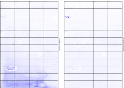
for the microarrays. These images can be quite noisy, the exact shape and intensity of the spots has to be determined and extracted from the background. Therefore, powerful image analysis software is required to extract good quality data from the images. Figure 2.1 shows background images extracted by an image analysis software. Some artifacts can easily be determined. Spots in the corresponding regions should be analyzed very carefully. Mostly, such spots are flagged by the image analysis software, and flagged values are ignored by later analysis programs.
Normalization of the raw data: The next step after the image analysis is the
normal-ization of the data. The goal of normalnormal-ization is to remove from the data systematic effects that are caused by the technical procedure rather than biological differences. In general, normalization consists of different steps: background correction, probe-level analysis (for oligonucleotide arrays), within-array normalization (for cDNA ar-rays), and between-array normalization. A review on microarray data normalization can be found in Quackenbush (2002).
22 2. Expression Data Analysis
z−range 31 to 457 (saturation 31, 457) z−range 44 to 1411 (saturation 44, 1411)
2.3 Analysis methods 23
cancer study (Lapointe et al., 2004) before and after (within-array) normalization. M denotes the logarithm of the expression ratio of the two channels while A denotes the logarithm of the average intensity.
Computation of differentially expressed genes: For many research questions, it is
of interest to find differentially expressed genes between two states. For instance, in pharmaceutical research expression levels for diseased and normal tissue samples are measured. The first apparent question is, which genes show different expression behavior between the sample groups. This problem boils down to distinguish random noise in the measurements from real biological differences. Furthermore, when the data are not or inappropriately normalized, systematic differences between arrays can arise. Thus, the computation of differentially expressed genes depends on the normalization step.
Clustering of genes or samples: Since the famous work by Eisen et al. (1998),
cluster-ing of genes or samples is another standard procedure for the analysis of microarray data. Generally, clustering of objects can provide a visualization of distances in high-dimensional spaces, e.g. as a dendrogram, and exhibit subgroups (clusters) where objects within subgroups are more similar to each other than objects from different subgroups. Clustering of genes organizes genes into groups with similar expression profiles. Often, these genes are functionally related (Eisen et al., 1998). Furthermore, clusters with profiles showing changes in regulation contain genes that are important in the experimental conditions under investigation. Clustering of samples can for instance exhibit disease subgroups with clinical relevance.
Sample classification: Sample classification provides a method for diagnosis of diseases.
Often, samples are classified using differentially expressed signature genes, therefore providing hints to the biological processes connected to the classification. Popu-lar techniques for classification include support vector machines and decision trees. Sample classification for disease diagnosis is of particular interest when it can be performed in early disease stages and when samples can be obtained by non-invasive methods such as blood samples.
Enrichment analysis: Enrichment analysis provides a simple and powerful method to
exploit context information in the form of predefined gene sets. Such a set could represent all proteins in a pathway or all genes that play a role in a certain biological process. The goal of the analysis is to identify gene sets that are enriched in genes that show an interesting expression pattern, for instance genes that are differentially expressed. This is usually accomplished by statistical tests, most often by Fisher’s
exact test or a χ2-test.
24 2. Expression Data Analysis
0 2 4 6 8 10 12 14
−10
−5
0
5
10
/home/proj/daten/Lapointe/padded_rawfiles//21081
A
M
0 2 4 6 8 10 12 14
−10
−5
0
5
10
/home/proj/daten/Lapointe/padded_rawfiles//21081
A
M
2.3 Analysis methods 25
2.3.1
Image analysis
The two most popular image analysis programs for microarray data, apart from the Affymetrix GeneChip software, are probably Spot, distributed by CSIRO Mathemati-cal and Information Sciences, Australia, and GenePix, by Axon Instruments, which also sells microarray scanners and other related hard- and software. GenePix includes not only the image analysis but also software for the control of the scanning process and has more or less become an industry standard. While GenePix is a stand-alone software that runs only on Windows platforms, Spot is a package for the R statistics environment (R Development Core Team, 2004). This allows an easy integration of results from the Spot software into other statistical methods implemented in R. There are many more soft-ware packages for the analysis of microarray images. A short comparison of such packages
can by found on Y. F. Leung’s functional genomics website1.
The main tasks for the image analysis software is to correctly estimate the shape and intensity of the spots as well as the background intensity. A review on image analysis methods can be found in Yang et al. (2001).
2.3.2
Normalization
Background correction
The image analysis software usually returns foreground- and background values for each spot. It is assumed that the foreground consists of two components, the signal from the bound cDNA molecules and noise from natural fluorescence, unspecific binding and the imaging process. The noise can be estimated from the background where no DNA was spotted. The simplest and most commonly used method for background correction is subtraction of the background intensities from the foreground intensities. Unfortunately, this leads to an increase of variance (fore- and background measurements both have vari-ance, the sum has a greater variance) and many negative intensity values that can not be handled by some subsequent methods. Therefore, other methods try to minimize the number of negative values and use more sophisticated methods for background correction. Kooperberg et al. (2002) for instance use a Bayesian method, while Edwards (2003) use background subtraction if the difference between foreground and background intensities is large and uses a smooth monotonic and positive function when the difference is small or negative.
Alternatively, the background correction step can simply be skipped which can of course lead to biased ratios in cDNA arrays if the background differs in the two channels.
Lo(w)ess normalization
The lowess or loess method can be employed to remove intensity-dependent biases from
two-channel microarray data. The name is derived from the term “locally weighted
1