5
XI
November 2017
Computational Electromagnetics: Techniques
and Applications
Sandip Mehta1, Anil Kumar Singh Raghav2
1, 2
Department of Electrical and Electronics Engineering, JIET Group of Institutions, Jodhpur
Abstract: This paper focuses on the concepts of computational techniques and its applications in the real world. Computational Electromagnetics (CEM) is widely used as a design tool for many electromagnetic problems. CEM is basically an interdisciplinary field which involves the solution of Maxwell's equations analytically using various methods of CEM and also determining the optimal method for a given problem. The first method described in this paper is the Finite difference method, which is more or less straight forward discretization of Maxwell's equation in differential form using field concept on a grade of unknown points. The second method is the Finite Element Method which is mainly used for time-harmonic problems, while the last method, the Method of Moments discretizes Maxwell’s equations in integral form. The applications of each of these methods is also discussed in this paper.
Keywords: Computational Electromagnetics (CEM), Maxwell's equation, Finite Element Method (FEM), Method of Moments (MOM), Finite Difference Method (FD)
I. INTRODUCTION
Today’s society is largely dependent on a variety of electromagnetic devices and systems including TV, mobiles, telephones, internet, satellites, computers, power system, microwave ovens, etc. Electromagnetic phenomena thus has a deep impact on modern society. The electromagnetic phenomena can be understood by electromagnetic field theory which describes the interactions between electric charges (at rest and in motion) by Maxwell’s equations developed in 1864. Analytical solutions in closed form are known for only a very limited number of special cases, which hardly ever are directly applicable to real-world applications. Instead, more or less crude approximations have been employed in various attempts to bridge the gap between theory and advanced applications.
The advent of computers has changed the ability to solve Maxwell’s equations in a profound way. With powerful computers at hand, it is now easy to use analytically simple methods that may require large amounts of computation. Such computational methods can treat large classes of problems without modifications of the computer algorithms or programs. The part of electromagnetics that deals with computational methods is known as Computational Electromagnetics, Computational Electrodynamics or Electromagnetic modelling. It is the process of modeling the interaction of electromagnetic fields with physical objects and the environment. It typically involves using computationally efficient approximations to Maxwell's equations and is used to calculate antenna performance electromagnetic compatibility, radar cross section and electromagnetic wave propagation when not in free space. A specific part of CEM deals with electromagnetic radiation scattered and absorbed by small particles.
The performance of CEM tools is increasing rapidly. One reason for this is the steady growth of computer capacity since last few decades. Besides, improvements in algorithms is another important reason. CEM allows for a faster and cheaper design process, where the use of expensive and time-consuming prototypes is minimized. These tools can also provide crucial information and understanding of a device’s electromagnetic operation, which may be difficult or even impossible to achieve by means of experiments or analytical calculations. It is only relatively recently that optimization by computation has been used for electromagnetic design problems.
The CEM methodology can be classified into two domains viz. time domain and frequency domain. Though Maxwell’s Curl equations are in time-domain, most electromagnetic instructions and research has taken place in frequency domain (assuming time harmonic behavior) the reason behind this being the slow growth of computers. The frequency domain approach is generally more tractable analytically and also the hardware available for modelling were confined to the frequency domain approach.[1][2]
(FEM), and the boundary element method (BEM), which is usually referred to, for historical reasons, as the method of moments (MoM) [2].
The finite-difference time-domain method was proposed by Yee [1] in 1967. The method of moments (MOM) was popularized among the electromagnetics community by Harrington [2] in 1968. There are other numerical methods which were developed from Variational methods, based on the so-called Euler´s Brachistochrone problem [3], and Variational calculus [3]. In the late 1960s, the finite element method was first applied to electromagnetics by Winslowin [1][2] in 1967. A review of methods used for CEM is found in a paper by Ney.M.Niziolek [4]in year 2009. Later on, S. Salon, Kiruba Jerry Selvaggi [5] presented a paper on CEM and silent motors. In 2013, Ricardo, Marco and Oriol [6] applied the Validation method in CEM simulations. In the same year, R. Douvenot, C. Morlaas and A. Chabory [7] presented their paper on theoretical studies of boundary conditions for parabolic equations. Application of FD in modeling of short gap electrostatic discharge was presented in a paper by Kazuhiro [8] in the year 2017. Application of FEM in reluctance machines for copper loss calculation is given by M. Al Eit and G. Krebs [9] in 2017. The rest of the paper is arranged as follows. The three CEM methods are introduced in section II, III, and IV respectively while their comparison is done in section V. The conclusions are presented in section VI.
II. FINITEDIFFERENCEMETHOD
Finite-difference (FD) is a numerical analysis technique used for modelling computational electrodynamics (finding approximate solutions to the associated system of differential equations). Since it is a time-domain method, FD solutions can cover a wide frequency range with a single simulation run, and treat nonlinear material properties in a natural way [10].
The FD method belongs to the general class of grid-based differential numerical modelling methods (finite difference methods). The time-dependent Maxwell's equations are discretised using central-difference approximations to the space and time partial derivatives. The resulting finite-difference equations are solved in either software or hardware. The electric field vector components in a volume of space are solved at a given instant in time; thereafter, the magnetic field vector components in the same spatial volume are solved; and the process is repeated over and over again until the desired transient or steady-state electromagnetic field behavior is fully evolved. Its principle is close to the numerical scheme used to solve ordinary differential equations. It is used to solve Maxwell's time dependent curl equation. Field is evolved by iterating Maxwell's equation in small time steps. In this method the derivatives are replaced in the equation using differential quotients (example Taylor series). The finite part of the Taylor series is used in the approximation [1],[10].
This highly versatile method is very useful for transient analysis. However, numerical problems with curved surface are difficult to be solved by this method. Further, this method is also not appropriate for small objects like modeling of thin wires. Also the efficiency is very low for highly resonating devices.
The Finite Difference Method is widely used in Wave Propagation, Microwave/Antenna, high-speed electronics, photonics, and biomedical problems.
III.FINITEELEMENTMETHOD
The finite element method (FEM) is used to find approximate solution of partial differential equations (PDE) and integral equations. The solution approach is based either on eliminating the time derivatives completely (steady state problems), or rendering the PDE into an equivalent ordinary differential equation, which is then solved using standard techniques such as finite differences, etc. In solving partial differential equations, the primary challenge is to create an equation which approximates the equation to be studied, but which is numerically stable, meaning that errors in the input data and intermediate calculations do not accumulate and destroy the meaning of the resulting output. The finite element method is a good choice for solving partial differential equations over complex domains or when the desired precision varies over the entire domain.
In this method, the area or field is divided into number of non-overlapping subareas or field called finite elements (triangles in 2D and tetra hydra in 3D). This method is best for eddy current calculations. It is best or well suited for problems having complex geometry. There are three different approach in formulating finite element method (FEM) problems. The approaches are as follows. The Direct Approach is the easiest out of these three approaches. It does not requires much knowledge of mathematics. However, only simple problems can be solved using this method.
The Weighted Residual Method involves two major steps for solving FEM problems. The approximate solution is assumed based on general behavior of variable (unknown) which satisfies boundary conditions. This solution is then substituted in the differential equation. However, it will not satisfy the differential equation; the resultant error generated is called residue. The residue is then made to vanish in some average sense to produce a system of algebraic equation. Thereafter, solving these algebraic equations gives approximate solution to the problem.
The Finite Element Method is best suited for problems having complex geometry. Computer codes for the formulation of FEM problems are easier and simple. The working domain or the application of this method is very vast. It is the most iterative method. In general it is a closed form solution which would permit one to examine system response to change in various parameters, is not produce. Solutions obtained via FEM are not appropriate they are approximate.
Remarkable advantage of FEM is the flexibility in terms of modelling any complicated geometry, distribution of media and easily solving problems associated with inhomogeneous medium. Use of this method gives sparse matrix equation (each element only interacts with elements in its own neighborhood). This method requires conversion of the entire domain into a mesh. If the problem is bounded, then normal procedure for solving FEM problems is applied. However, if the problem is unbounded, then the following software viz. ABC, PML or FE-BI may be applied.
The FEM method can be applied for solving both linear and nonlinear, and, 2-D/3-D problems. Apart from being applied to problems in time-domain, it can also be used for solving problems in the frequency domain. This technique is widely used in aeronautical, biomechanical and automotive industries.
IV.METHODOFMOMENTS(BOUNDARYELEMENTMETHOD)
The Method of Moments (MOM) or Boundary Element method (BEM) is a numerical computational method of solving linear partial differential equations which have been formulated as integral equations (i.e. in boundary integral form). It can be applied in many areas of engineering and science including fluid mechanics, acoustics, electromagnetic and fracture mechanics.
Boundary integral equations are a classical tool for the analysis of boundary value problems for partial differential equations. The term “boundary element method” (BEM) denotes any method for the approximate numerical solution of these boundary integral equations. The approximate solution of the boundary value problem obtained by BEM has the distinguishing feature that it is an exact solution of the differential equation in the domain and is parameterized by a finite set of parameters living on the boundary. The step in formulation of the MOM problems are as follows:
1) Find derivative of the appropriate integral equations.
2) Discretize this to form matrix equation using basic expansion function and weighting functions.
3) Evaluate these matrix elements.
4) Solve matrix to obtain final results.
Only the boundary of the domain needs to be discretised. Especially in two dimensions where the boundary is just a curve, this allows very simple data input and storage methods. Exterior problems with unbounded domains but bounded boundaries are handled as easily as interior problems. In some applications, the physically relevant data are given not by the solution in the interior of the domain but rather by the boundary values of the solution or its derivatives. These data can be obtained directly from the solution of boundary integral equations; whereas boundary values obtained from FEM solutions are in general not very accurate. The solution in the interior of the domain is approximated with a rather high convergence rate and moreover, the same rate of convergence holds for all derivatives of any order of the solution in the domain. There are difficulties, however, if the solution has to be evaluated close to, but not on the boundary. This method does not yield good results for problems related to materials exhibiting dispersion and the dielectric materials. It has long and tedious formulation. This method is inefficient for problems with volumetrically complex structures.
The MOM method is applicable to many EM-related application areas such as Electrostatic problems, Wire antennas and scatters, Scattering and radiation from bodies of revolution or bodies of arbitrary shape, Transmission lines, Aperture problems, Biomedical problems, Mathematical model, Boundary integral equation, Boundary elements, Discrete equations, Solution of the linear system, Interpretation.
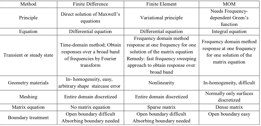
V. COMPARISONOFVARIOUSMETHODSOFCOMPUTATIONALELECTROMAGNETICS
Table 1. Comparison of the three CEM methods
Method Finite Difference Finite Element MOM
Principle Direct solution of Maxwell’s
equations Variational principle
Needs Frequency- dependent Green’s
function
Equation Differential equation Differential equation Integral equation
Transient or steady state
Time-domain method; Obtain responses over a broad band
of frequencies by Fourier transform
Frequency domain method response at one frequency for one
solution of the matrix equation Remedy: fast frequency sweeping
approach to obtain response over broad band
Frequency domain method response at one frequency
for one solution of the matrix equation
Geometry materials In- homogeneity, easy,
arbitrary shape staircase error Nonlinearity In-homogeneity, difficult
Meshing Entire domain discretized Entire domain discretized Normally only surfaces
discretized
Matrix equation No matrix equation Sparse matrix Dense matrix
Boundary treatment Open boundary difficult
Absorbing boundary needed
Open boundary difficult Absorbing boundary needed
Open boundary easy
VI.CONCLUSION
The three methods of Computational Electromagnetics viz. the Finite Difference Method (FD), the Finite Element Method (FEM) and the Method of Moments (MOM) have been introduced in this paper along with the applications, advantages and drawbacks. A comparison has been made at the end based upon various parameters.
Each method has its own area of applications. There is no single method that can cater to all problems. Based on the problem, one particular method may be adopted. Comparing the performance of FD, FEM and MOM would give better insight into CEM.
Future studies and research would be in the direction of hybrid techniques that have been on the rise recently which has resulted in achieving higher efficiency in terms of computational time, memory storage and accuracy.
REFERENCES
[1] Thomas Rylander, Anders Bondeson and Par Ingelstrom, “Computational Electromagnetics”, 2nd edition, Springer, 2013. [2] Richard C. Booton Jr., “Computational Methods for Elecromagnetics and Microwaves”, A Wiley- Interscience publication, 1926. [3] Robert Cook, “Concepts and application of Finite Element Analysis”, 2nd edition John Wiley and Sons, 1989.
[4] M. Niziolek, “Review of Methods used for Computational Electromagnetics” Electrodynamic and mechatronics, 2nd Internationalconference, 2009.
[5] S. Salon, M. V K Chari, Kiruba Sivasubramaniam, O. Mun Kwon, Jerry Selvaggi “Computational electromagnetics and the search for quiet motors”, Journal IEEE Transactions on Magnetics, vol. 45, 2009.
[6] Ricardo Jauregui, OriolVentosa, and Marco Kunze, ”Aalysis of pre-processing techniques when using validation methods in CEM simulations” IET Science, Measurement and technology, vol. 7, issue 3, 2013.
[7] R. Douvenot, C. Morlaas, and A. Chabory, “A theoretical study of the boundary conditions for parabolic equations,” IEEE ASP Topical Conference on Antennas and Propagation in wireless comm., 2013.
[8] Kazuhiro Fujita, “Efficient finite difference time domain modeling of short gap electrostatic discharge caused in the vicinity of complex electronic system” IEEE International Conference on CEM, 2017.
[9] M. Al Eit, P. Dular, F. Bouillault, and G Krebs,” Pertubation Finite Elements method for Efficient Copper Losses Calculation in Switched reluctance machines” IEEE Trans. Magnetics, vol. 53, issue 6, 2017.