Normalization and analysis of DNA microarray data by self consistency and local regression

comment

reviews

reports

deposited research

interactions

information

refereed research

Research

Normalization and analysis of DNA microarray data by

self-consistency and local regression

Thomas B Kepler*, Lynn Crosby

†

_{and Kevin T Morgan}

‡

Addresses: *Santa Fe Institute, Santa Fe, NM 87501, USA. †_{University of North Carolina Curriculum in Toxicology, US Environmental} Protection Agency, Research Triangle Park, NC 27711, USA. ‡_{Toxicogenomics-Mechanisms, Department of Safety Assessment,} GlaxoSmithKline, 5 Moore Drive, Research Triangle Park, NC 27709, USA.

Correspondence: Thomas B Kepler. E-mail: kepler@santafe.edu

Abstract

Background:With the advent of DNA hybridization microarrays comes the remarkable ability, in principle, to simultaneously monitor the expression levels of thousands of genes. The quantiative comparison of two or more microarrays can reveal, for example, the distinct patterns of gene expression that define different cellular phenotypes or the genes induced in the cellular response to insult or changing environmental conditions. Normalization of the measured intensities is a prerequisite of such comparisons, and indeed, of any statistical analysis, yet insufficient attention has been paid to its systematic study. The most straightforward normalization techniques in use rest on the implicit assumption of linear response between true expression level and output intensity. We find that these assumptions are not generally met, and that these simple methods can be improved.

Results: We have developed a robust semi-parametric normalization technique based on the assumption that the large majority of genes will not have their relative expression levels changed from one treatment group to the next, and on the assumption that departures of the response from linearity are small and slowly varying. We use local regression to estimate the normalized expression levels as well as the expression level-dependent error variance.

Conclusions: We illustrate the use of this technique in a comparison of the expression profiles of cultured rat mesothelioma cells under control and under treatment with potassium bromate, validated using quantitative PCR on a selected set of genes. We tested the method using data simulated under various error models and find that it performs well.

Published: 28 June 2002

GenomeBiology2002, 3(7):research0037.1–0037.12

The electronic version of this article is the complete one and can be found online at http://genomebiology.com/2002/3/7/research/0037 © 2002 Kepler et al., licensee BioMed Central Ltd

(Print ISSN 1465-6906; Online ISSN 1465-6914)

Received: 20 February 2002 Revised: 21 March 2002 Accepted: 17 April 2002

Background

Among the most fascinating open questions in biology today are those associated with the global regulation of gene expres-sion, itself the basis for the unfolding of the developmental program, the cellular response to insult and changes in the

thousands of genes - sufficient numbers to measure the expression of all of the genes in many organisms, as is now being done in the eukaryote Saccharomyces cerevisiae[7,8].

If we designate the intensity of a given spot in the microarray as Iand the abundance of the corresponding mRNA in the target solution as A, we have, under ideal circumstances,

I= N A+ error (1)

where Nis a constant, unknown normalization factor. When comparing two different sets of intensities, these factors (or at least their relative sizes) must be determined in order to make a relative comparison of the abundances A.

The simple normalization techniques commonly used at this time assume Equation 1. Under these conditions, normaliza-tion amounts to the estimanormaliza-tion of the single multiplicative constant Nfor each array. This task can be implemented by whole-array methods, using the median or mean of the spot intensities or by the inclusion of control mRNA.

We have found in a variety of different hybridization systems that the response function is neither sufficiently linear, nor consistent among replicate assays; the relationship between the intensity and the abundance is more complicated than that found in Equation 1. There may, for example, be a con-stant term, interpretable as background:

I= N0+ N1A+ error, (2)

or the intensity may saturate at large abundance:

I= —————N1A

1 + N2A+ error. (3)

Both these situations render simple ratio normalizations inadequate. The problems are not obviated by the use of ‘housekeeping’ genes as controls. First, their quantitative stability is not a prioriassured, nor has such stability been demonstrated empirically, and second, even if such genes were found, the nonlinearity of the response is not addressed by this technique. Neither can extrinsic controls (such as bacterial mRNA spiked into human targets) ensure adequate normalization, as the relative concentration of control to target mRNA cannot itself be known with sufficient accu-racy. Even simultaneous two-color probes on the same microarray do not eliminate the problems of normalization because of variation in the relative activity and incorporation of the two fluorescent dyes.

One possible approach to the normalization problem would be to obtain detailed quantitative understanding of each step in the process in order to develop a mechanistic model for the response function. This approach is almost certainly important for the optimization of array design, but may not be necessary for data analysis. Alternatively, one may use the vast quantity

of data generated and the assumption of self-consistency to estimate the response function semi-parametrically.

We have pursued the latter path. Our approach does not rely on the consistency of an extrinsic marker or the stability of expression for any given set of genes or on the correctness of

an a priori model for the response, but rather upon the

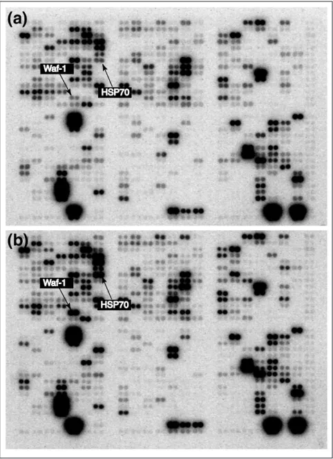
assumption that the majority of genes in any given compari-son will be expressed at constant relative levels (Figure 1); only a minority of genes will have their expression levels affected appreciably. Thus, we normalize pairs or groups of arrays relative to each other by maximizing the consistency of relative expression levels among them.

The underlying idea is that the majority of genes will not have their expression levels changed appreciably from one ment to the next (Figure 1). Clearly, there may be some treat-ment pairs for which this is not a reasonable assumption, but we argue that as long as the cell is alive, the basic mechanism of cell maintenance must continue; the relevant gene prod-ucts must be kept at relatively stable levels. This approach can be viewed as a generalization of the method of using ‘housekeeping’ genes to normalize the array. But rather than choosing a particular set of genes beforehand, assuming that their expression levels are constant across treatments, we assume that there is a stable background pattern of activity, that there is a transcriptional ‘core’, and identify its con-stituent genes statistically for each experiment.

The essential contrast between our method based on self-consistency and that based on control genes determined

a prioriis concisely captured in the following flow diagrams.

Normalization by controls identified a priori

1. Assume that some genes will not change under the treat-ment under investigation.

2. Identify these core genes in advance of the experiment (housekeeping genes, extrinsic controls)

3. Normalize all genes against these genes assuming they do not change

4. Done.

Normalization by self-consistency

1. Assume that some genes will not change under the treat-ment under investigation.

2. Initially designate all genes as core genes.

3. Normalize (provisionally) all genes against the core genes under the assumption that the true abundance of the core genes does not change.

comment

reviews

reports

deposited research

interactions

information

refereed research

5. If the new core differs from the previous core, then go to step 3.

6. Else: done.

Modeling and estimation

We concentrate here on the experimental design with two treatment groups and two or more replicate arrays per group. Generalization to more than two groups is straight-forward. Comparisons made without replicate arrays are also possible, and much of the methodology discussed here can be applied in that case as well, but the lack of true repli-cates introduces unique non-trivial problems that will not be considered here.

The basic model

Let Yijk = logIijk denote the logarithm of the measured intensity of the kth spot in the jth replicate assay of the ith

treatment group. Thus, kranges from 1 to G, the number of genes per array, jranges from 1 to ri, the number of repli-cate arrays within the ith treatment group, and i takes values from 1 to the number of treatment groups. The examples in this paper use two treatment groups. The loga-rithmic transformation converts a multiplicative normaliza-tion constant to an additive normalizanormaliza-tion constant. We also find that this transformation renders the error vari-ances more homogeneous than they are in the untrans-formed data. Then the error model corresponding to Equation 1 is:

Yijk= nij+ ak+ dik+ s0eijk (4)

where the nij= logNijare now the normalization constants, ak+ dik= logAikare the mean log relative abundance and the differential treatment effects, respectively, and s0 is the

error standard deviation. The treatment effects, dd, are the quantities of most direct interest for comparing expression profiles. We assume that the residuals eijkare independent and identically distributed and have zero mean and unit variance. For the significance tests below, we will further assume that the errors are normally distributed.

Estimation by self-consistency

Estimation of the parameters in Equation 4 is carried out in an iteratively reweighted least-squares (IRLS) procedures. First, let ck indicate the assignment of the kth gene to the core set: ck= 0 if gene kis not in the core and ck= 1/rGif gene kis in the core, where rGis the number of genes in the core. The vector cis thus normalized: åkck= 1. These indica-tors play the role of weights in an IRLS. Although they do depend on other estimated parameters, in each iteration the weights are treated as constants, depending only on parame-ter estimates from the previous iparame-teration.

The notion of self-consistency arises in the combined processes of identifying the core and normalizing the data: the choice of genes belonging to the core depends on the normalization, and the optimal normalization depends on which genes are identified with the core.

We start by minimizing the core sum of squares (SSC):

SSC =

兺

ijk ck 冢Yijk- nij - ak冣

2 ₍₅₎

over aand n. Note that one can add a constant to nand sub-tract the same constant from awithout changing SSC. This invariance corresponds to our inability to estimate absolute abundances, but relative abundances only. We therefore enforce an ‘identifiability’ constraint: åkak= 0. The mini-mization gives:

ak= Y–..k- Y–…

nij = Y–… +

兺

k ck 冢Yijk- Y–..k冣 (6)

Figure 1

where aand nare the estimators for aand n, respectively; overbars indicate averages over the dotted subscripts, for example, ^Yij= 1/G兺Gk=1Yijk.

The normalized and scaled data are now given by

Y^ijk= Yijk - nij

= Yijk - Y–… -

兺

k ck 冢Yijk- Y–..k冣 (7)

Note that if all of the genes are placed in the core, we have

Y^ijk= Yijk - Y–ij. (8)

as expected.

Now we estimate the differential treatment effects by mini-mizing the residual sum of squares,

SS =

兺

ijk 冢Yijk- nij - ak - dik冣

2 ₍₉₎

of the normalized data over dd, yielding

dik= Y–i·k- Y–..k -

兺

G

k¢=1 ck¢冢Y–i·k¢- Y–..k¢冣 (10)

Note that the matrix, d, of differential treatment effects obeys åiridik= 0, as we would hope.

Self-consistency requires that the vector of core indicators c

depend on the estimated differential treatment effects, d. We have tried several methods for implementing an appro-priate dependence and find that one of the simplest schemes works very well. We simply fix the proportion rof genes in the core, rank the genes by the square of the estimated dif-ferential treatment effect åiridik2and remove from the core for the next iteration those genes in the 1 - r quantile.

0 for 兺iridik2⬎q

ck =

再

——

rG for 兺iridik2ⱕq

where qis a threshold chosen to ensure that a fixed propor-tion rof genes are designated core genes. Note that a possi-ble improvement to the algorithm might be found by appropriate optimization of rrather than simply fixing it in advance.

We carry out the estimation iteratively. We start with ck= 1/G for all k (all genes in the core) and estimate dikby Equa-tion 10. We then update c according to Equation 11 and repeat the estimation of ddwith this new c. We stop when c

does not change from one iteration to the next.

The local regression model

What we find in the analysis of experimental data, however, is that Equation 1 with Nconstant is not adequately realistic. A more flexible approach that covers the contingencies of Equations 1-3 and many others, is to generalize Equation 4 to

Yijk= nij (ak) + ak+ dik+ s(ak)eijk. (12)

where nijis the normalization function, now assumed explic-itly to depend on the mean log abundance ak. The function

s, which scales the error variance, describes the hetero-scedasticity, or non-constancy of the variance, which we here assume depends only on the mean log intensity level. The two functions are constrained to vary slowly and thus can be estimated by local regression.

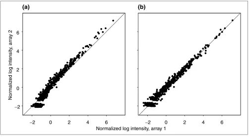
If Equation 4 is used to estimate the normalization, the departures from linearity manifest themselves as systematic bias in the residuals (Figure 2). In all the data we have exam-ined, the resulting biases are small and slowly-varying func-tion of the mean log intensity, and so can be estimated using local regression on a, the estimator for the mean log abun-dance. It should be noted that an additive component of the variability with non-zero expectation, in addition to the mul-tiplicative noise (Equation 2) can, when the logarithmic transformation is applied, lead to such nonlinear response curves. Our approach here is to develop a method flexible enough to allow for all sources of nonlinearity, including additive noise. We demonstrate the validity of this method for these formally mis-specified models in our simulation studies below.

Estimation of both the normalization function, n, and of the heteroscedasticity sis carried out by local regression.

Local regression

Local regression is a generalization of the intuitive idea of smoothing by using a moving average. In local regression, one goes beyond computing the local average of a set of mea-sured points by estimating, at each value of the predictor variables, all of the coefficients in a Pth-order regression in which the regression coefficients themselves are slowly varying functions of the predictor variable. Computation of a moving average is thus a zeroth order local regression. The availability of inexpensive powerful computing has sparked renewed interest in local regression techniques and its theo-retical underpinnings have been extensively elucidated [9-11].

Modeling a response function vas a function of a predictor u

via local regression proceeds in two steps. First, we estimate a function of two variables uand u¢,

f(u¢;b(u)) = b0(u) + b1(u)(u - u¢) + … + bP(u)(u - u¢)P. (13)

with u, the quantitative rates of change specified by a para-meter introduced below. Second, we estimate v(u) as

v

^(u) = f(u; b(u)) (14)

where bis the vector of estimators for b. In other words, we estimate the coefficients and evaluate the function at u¢=u. The terms of order greater than 0 vanish, but the estimates for the remaining zeroth-order terms depend nevertheless on the estimated higher-order coefficients, as follows. Given a dataset consisting of npairs (ui,vi), iÎ(1,...,n), we estimate the coeffi-cients at a point u(not necessarily corresponding to any uiin the dataset), by minimizing a weighted sum-of-squares over b:

SS(u) =

兺

i wi(u)(vi - f(ui;b(u)))

2 ₍₁₅₎

The weighting functions ware given by

wi(u) = W

冢

冣

where Wis a symmetric function having a simple maximum at the origin, strictly decreasing on [0,1] and vanishing for

u³1. For our application in this paper, we use the efficiently computed tricube function

ck(1 - |x|3)3 for |x| < 1

W(x) =

再

0 otherwise

The function his known as the bandwidth, and controls just how slowly fvaries with u. We choose the bandwidth so as to give equal span at all points u. The span is defined as the proportion of points uicontained in a ball of radius h(u). This choice of bandwidth function is used in Loess regres-sion [11]. For all of the computations in this paper, we have used a span of 0.5.

Minimization of Equation 15 over the coefficient vector b(u) results in linear equations of the form

bi(u) = Li(u)v (18)

Where Liis the linear operator appropriate to the ith coeffi-cient and vis the vector with components vk. Note that the Li depends on the order Pof the local regression. For any given value of P, the Lican be explicitly written down, but quickly become algebraically complicated.

The local regression estimate of f(u;b(u)) is

f(u; b(u)) = b0(u) = L0(u)v (19)

comment

reviews

reports

deposited research

interactions

information

refereed research

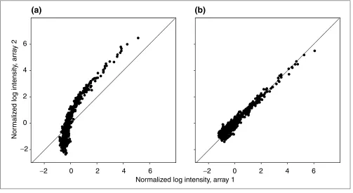
Figure 2

The normalized log intensity in a pair of replicate arrays. (a)Data normalized by subtracting the mean over all spots; that is, no bias removal. (b)Data normalized by estimating the normalization function using local regression and then subtracting the inferred bias, as described in the text.

−

2

0

2

4

6

−

2

0

2

4

6

Nor

maliz

ed log intensity

, arr

a

y 2

−

2

0

2

4

6

Normalized log intensity, array 1

(a)

(b)

Because of this linearity, the sampling distributions for these coefficients are known and we can compute their sampling variances in a straightforward manner [11].

To adapt this method to the problem of normalization, and simultaneously to implement self-consistency, we take for the weighting functions the product of a tricube and a core indicator:

ck冢1 - |———ah- (aa)k| 3

冣3 for |a- ak| < h(a)

wk(a) =

再

0 otherwise

where ckis the core indicator as given in Equation 11 and the akare given by Equation 6. In these terms, the local regres-sion estimate nof nis given by

nij(ak)= Y–… +

兺

k¢Lk¢

0 _(a

k) (Yijk¢ - Y..k¢) (21)

with the normalized data given by

Y^ijk= Yijk - nij (ak) (22)

and the differential treatment effects by

dik= Y–i·k- Y–..k -

兺

k¢ Lk¢

0 _(a

k) (Yijk¢ - Y..k¢). (23)

Again, we have åiridik = 0. The core indicator vector cis then iterated to fixation as described in the previous section but with åiridik2 compared against qs2(ak) where s2(a) is the estimated local variance, discussed in the next section.

Local variance estimation

In addition to local nonlinearities in the response curve, we also find that the data are heteroscedastic: the error variance shows a clear dependence on the estimated abundance. The logarithmic transformation removes a substantial part of this dependence, but does not flatten it out entirely. One might try

an a priori accounting of the sources of error and thereby

provide a parametric model for it, but the number of poten-tial error sources is large, so we instead choose a flexible error model and estimate local variance by again using local regres-sion. The technique involves computing the local likelihood and the effective residual degrees of freedom and is described in detail in [11]. Their ratio of the local likelihood and the effective degrees of freedom provides a smooth estimate of the local variance. The estimated residuals are not strictly linear functions of Ybecause of the implicit dependence of the indicator vector con the data Yand because of our use of the estimator a, rather than a strictly independent variable, as the predictor for the local regression. We expect these cor-rections due to nonlinearities to be small and thus neglect them in our estimates of the local variance.

At this stage, we have computed a first-order approximate solution for the estimation problem. We may now perform another iteration (in addition to the iterated solution for the core indicator c) to improve the approximation, reweighting the data by the inverse of the estimated local variance. Our experience, however, has been that the first-order correc-tions are sufficient and the higher-order correccorrec-tions are more difficult to compute and make little difference in the final analysis. For the applications and validation tests that follow, we use just the first-order corrections.

Pairwise expression-level comparisons

We perform individual pairwise hypothesis tests for each spot in the array by computing the statistic

d1k- d2k

zk= ———————————— (24)

s(ak) 兹1/r1 + 1/r2

where s(ak) is the square-root of the local variance at the mean relative expression value ak. We test zas a standard normal under the null hypothesis of no expression difference.

Validation

We illustrate the use of the computational methods by fixing r= 0.9 and applying them to data generated in an experi-ment carried out on cultured, spontaneously immortalized rat peritoneal mesothelial cells to determine the transcrip-tional effects of treatment with potassium bromate. The data consist of measured intensities of G = 596 genes from each of four arrays: two replicates r1 = r2 = 2 in each of two

treat-ment groups. A complete discussion of the biological results obtained in these experiments can be found in [12].

Results and discussion

B-cell lymphoma 2 (Bcl-2), and the pro-apoptotic Bcl-2-associated X protein n (bax n), Bcl-XL/Bcl-2 associated death promoter homolog (Bad) and Bcl-2 related ovarian killer protein (bok) (at 12 hours), and cell-cycle control ele-ments known as cyclins (at 4 and 12 hours), were downregu-lated. Several genes that inhibit the cell from entering the cell cycle were increased significantly at both time points.

Confirmation by quantitative PCR

Quantitative PCR analysis confirmed nine gene changes. The tenth, PLA2, could not be confirmed because of lack of signal in both treatment groups and was therefore likely to be due to a problem in the PCR for that gene [12].

Morphologic analysis revealed complete mitotic arrest by 4 hours post-exposure, with increased numbers of con-densed cells with pyknotic nuclei, believed to be apoptotic. Strong HO-1-specific staining was observed in treated cells, whereas control cells showed weak nonspecific staining, or no staining at all.

Statistical characteristics of the data

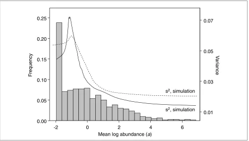
A histogram of mean log spot intensities (Figure 3) shows that nearly a quarter of the 596 spots on the array show little or no signal. The remainder of the distribution shows a very

gradual maximum followed by a long tail skewing the distri-bution to the right. The total range is about 9 (natural) logs, corresponding to approximately 9,000-fold change from highest intensity to ‘background’.

The estimated variance of the log intensities increases from the lowest log intensities for about one (natural) log to peak at a value of about 0.25 and then decreases to asymptote at about 0.04 for intense spots. This suggests that the error is domi-nated by different sources in the two intensity regimes. Fur-thermore, the fact that the variance of the log intensity decreases for large intensities indicates that the variance scales like aq_{, where q< 2. q= 2 corresponds to lognormal behavior} with constant coefficient of variation and q = 1 corresponds to the Poisson-like behavior of independent counting processes.

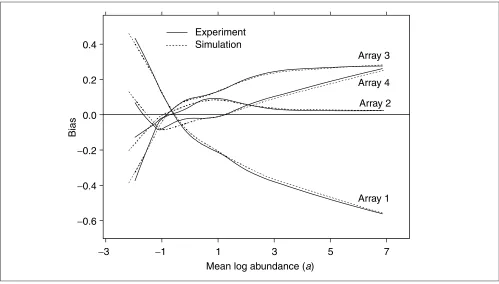
The four arrays in this study also showed non-negligible bias (Figure 4). The root-mean-square (RMS) bias over all four arrays was 17.5 x 10-2_{. This should be compared to the}

esti-mated standard deviation of the residuals after bias removal of 19.2 x 10-2_{; it is clearly comparable. This bias is not likely}

not to be an artifact of the fitting procedure. Application of the fitting procedure to simulated data without bias (see below) results in a range of RMS bias that is much smaller than that seen in the real data (Tables 1-3).

comment

reviews

reports

deposited research

interactions

information

refereed research

Figure 3

Histogram of estimated mean log abundance levels, a_k, and local variance (solid line) from the potassium bromate experiment. This distribution of xand this local variance curve were used as input for the simulation studies. The dashed curve gives the variance estimated in a randomly chosen member of the simulation datasets.

-2

0

2

4

6

Mean log abundance (a)

0.00

0.05

0.10

0.15

0.20

0.25

V

ar

iance

0.01

0.03

0.05

0.07

F

requency

s

_{, simulation}

In addition to the experiments reported here, we have exam-ined data from several other microarray platforms and find that in terms of the heteroscedasticity and apparent bias, they are qualitatively similar (not shown).

Simulation studies

To determine the reliability of our methods, we generated simulated data under a number of models based on the sta-tistical characteristics of the data obtained in our hybridization experiments. All of the simulated data was produced using FORTRAN programs calling IMSL subrou-tines for sorting, cubic spline interpolation and random number generation.

For each model and each set of conditions we ran 100 inde-pendent realizations. The data from each of these realiza-tions was used as input to our normalization routines, which performed normalizations in two ways. First, we normalized according to Equations 4, 10 and 6, that is, without bias removal and without accounting for heteroscedasticity; this procedure is referred to as ‘naive’. Then, we normalized according to Equations 12, 21 and 23 and r= 0.9 with bias removal and estimation of heteroscedasticity. The software that implements the latter method is referred to as NoSe-CoLoR, for Normalization by Self-Consistency and Local Regression [13]. For judging the relative performance of the

two methods, we recorded the number of true positives and the number of false positives for each simulated dataset.

Homoscedastic error model

In the first set of tests, the data were generated by simula-tions of the model

Yijk= n0ij+ qnij(ak) + ak+ dik + s0eijk (25)

where the values for n0

ijwere generated as normals with mean 0 and standard deviation 0.2, the ak were taken to be the values akestimated from the experimental data, s20= 0.039

(this is the value estimated from the experimental data, treated as homoscedastic) and eijkwere generated as stan-dard normal. The treatment effects were generated by choos-ing at random a fixed number of genes pG(10% or 20% of the total number G) and within this set, letting d1k= tklogf and d2k= 0. Outside this set, dik= 0. Here, tkare indepen-dently drawn from {-1,1} with equal probability, and fis the ‘fold change’, or ratio of expression level between treated and control groups.

The function nij(a) representing nonlinearity and bias was taken to be proportional to the corresponding function nij estimated in the above data analysis (Figure 4) and com-pleted by cubic spline interpolation. The constant of

Figure 4

Biases in the four arrays in the potassium bromate experiment (solid lines). These biases were then used as input to the data simulation as described in the text. A simulation dataset was chosen at random and biases were estimated from it (dashed lines).

−

3

−

1

1

3

5

7

Mean log abundance (a)

Bias

Array 1

Experiment

Simulation

Array 2

Array 4

Array 3

−

0.6

−

0.4

proportionality, designated q in the tables, regulates the size of the bias.

What we find (Table 1) is that the power of the test for the naive analysis is diminished by the presence of bias. For the local-regression analysis (NoSeCoLoR), the power is unaffected by the presence of bias. Furthermore, when the proportion, p, of affected genes among all genes is small (p= 10%), the power of the two methods is about the same. When p= 20%, the naive method has slightly better power when bias is absent.

Heteroscedastic error model

As discussed above, even the log-transformed data are not homoscedastic, but have variance that varies with the mean intensity level. The second set of simulations is similar to the first, but differs in that the constant s0in Equation 25 is

replaced by the function s(a) estimated from the Clontech array experiments (Figure 4). All other details are as for the previous simulation.

In this case (Table 2), we find as before that bias diminishes the power of the naive procedure, but not that of NoSe-CoLoR. In addition, the rate of false positives is now notably high for the naive method. NoSeCoLoR yields consistently

smaller false-positive rates, although when large proportions of genes are affected and have large effect size, the rate of false positives with NoSeCoLoR is also larger than nominal.

Compound error model

The model given by Equation 12 is intended to be flexible and to be a reasonable approximation to a variety of models. One particularly common source of nonlinearity is additive error (on the untransformed data), or background with non-zero mean (Equation 2). We have therefore simulated data according to a model given by

Iijk= exp {ak+ nij+ dik + eijk} + exp {zij+ hijk} (26)

comment

reviews

reports

deposited research

interactions

information

refereed research

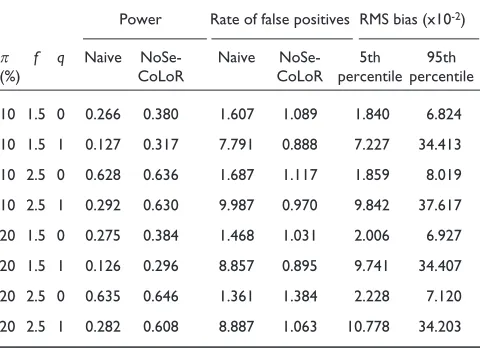
Table 1

Assessment of algorithm performance on data simulated according to the homoscedastic error model

Power Rate of false positives RMS bias (x10-2₎

p f q Naive NoSe- Naive NoSe- 5th 95th

(%) CoLoR CoLoR percentile percentile

10 1.5 0 0.318 0.315 1.024 1.035 0.937 1.710 10 1.5 1 0.127 0.300 0.929 0.933 16.559 17.872 10 2.5 0 0.989 0.974 1.004 1.181 1.524 3.292 10 2.5 1 0.689 0.971 0.955 0.968 15.776 17.163 20 1.5 0 0.327 0.314 0.975 1.002 1.079 2.226 20 1.5 1 0.129 0.295 0.883 0.973 16.380 17.742 20 2.5 0 0.985 0.939 1.000 1.662 3.359 5.763 20 2.5 1 0.684 0.941 0.889 1.298 15.279 16.823 The proportion,p, among all genes of those for which the expression level has been changed is either 10% or 20%. The ratio, f, of treated expression level to mean control expression level is varied between 1.5 and 2.5. The bias multiplier qis either zero (no bias) or 1 (bias as measured in the analysis of the real data). The power is the mean number of correct discriminations achieved in the test divided by the number of true changes (59 and 119 for p= 10% and p= 20%, respectively). The false-positive score is the mean number of incorrect discriminations divided by the expected number at the nominal type-I error rate of 0.01. The expected number of false positives is 5.4 when p= 10% and 4.8 when

p= 20%. The RMS bias is computed from the bias as estimated as described in the text. Reported here are the 5th and 95th percentiles over the simulated datasets.

Table 2

Assessment of algorithm performance on data simulated according to the heteroscedastic error model (Equation 26)

Power Rate of false positives RMS bias (x10-2₎

p f q Naive NoSe- Naive NoSe- 5th 95th

(%) CoLoR CoLoR percentile percentile

10 1.5 0 0.312 0.346 1.577 0.890 0.933 1.669 10 1.5 1 0.130 0.342 0.775 0.784 16.536 17.763 10 2.5 0 0.982 0.939 1.482 0.970 1.474 3.447 10 2.5 1 0.683 0.939 0.749 0.855 15.740 17.271 20 1.5 0 0.313 0.345 1.600 0.878 0.930 2.091 20 1.5 1 0.128 0.324 0.784 0.803 16.320 17.722 20 2.5 0 0.983 0.905 1.560 1.367 3.113 5.967 20 2.5 1 0.685 0.909 0.751 1.078 15.299 16.821 Details as in Table 1.

Table 3

Assessment of algorithm performance on data simulated according to a model with homoscedastic multiplicative error plus additive (background) error

Power Rate of false positives RMS bias (x10-2₎

p f q Naive NoSe- Naive NoSe- 5th 95th

(%) CoLoR CoLoR percentile percentile

where the terms a, n, dand ehave the meanings assigned above and are computed as in the first simulation. In partic-ular, ehas zero mean and constant variance with s= 0.2. The second exponential represents an additive background. This background is modeled as lognormal. The component zijcommon to all spots in an array is chosen as a normal random deviate with mean zero and standard deviation q. Differences in z from one array to the other can create apparent biases in the log-transformed data (Figure 5). The gene-specific term in the background hijkhas mean zero and standard deviation 0.2.

It is in this simulation that the naive method fails most dra-matically. For all datasets, the naive method gives false-posi-tive rates significantly greater than nominal, some as much as ten-fold higher than nominal. NoSeCoLoR has much better error rates, although as seen before, performance starts to suffer when larger numbers of spots are affected. The power of comparisons using NoSeCoLoR is again much more resistant to changes in the effective bias level (c in Table 3) than is the naive method.

Conclusions

We have presented a method for normalizing microarray data that relies on the statistical consistency of relative

expression levels among a core set of genes that is not identi-fied in advance, but inferred from the data itself. The nor-malization and variance estimation are both performed using local regression. We are then able to perform standard comparison tests. This technique reveals biologically plausi-ble expression-level differences between control mesothe-liomas and mesothemesothe-liomas treated with a potent inducer of oxidative stress. The expression changes identified by our normalization methodology were confirmed by quantitative PCR in all cases but one where there was no detectable PCR amplification at all.

Our simulation studies show that our normalization tech-nique performs well. The worst case occurs when the response curve is perfectly linear, the variance constant and a large proportion of genes experiences sizable expression-level changes. Under these conditions, our method has a false-positive rate somewhat greater than nominal and self-consistent normalization without local regression performs slightly better than that with local regression. On the other hand, our method is insensitive to bias and heteroscedastic-ity, both of which have a significant deleterious effect on the naive method. Furthermore, bias and heteroscedasticity are both measurably present in all data that we have examined from microarrays from a number of different manufacturers and from several different laboratories. In these cases, local

Figure 5

The normalized log intensities from simulated data generated according to Equation 26. (a) The data normalized without local regression, as in Figure 1.

(b)The same data normalized using local regression for bias removal. Note that the apparent curvature is induced simply by adding a background term with non-zero expectation.

−

2

0

2

4

6

−

2

0

2

4

6

Normalized log intensity, array 1

−

2

0

2

4

6

Nor

maliz

ed log intensity

, arr

a

y 2

regression performs better than self-consistency alone. When the data are generated by an additive-plus-multiplica-tive error model, the naive method completely breaks down, whereas our method continues to perform well.

We have applied these methods to the analysis of microarray data in toxicogenomic studies [12,14], where the results made good biological sense and, where relevant, were con-firmed by subsequent experimentation. All data-analytic techniques benefit from extensive use and assessment using several platforms and diverse biological systems. To facili-tate this process for the methods described here, and to provide them to the interested research community, we have made the software used to implement them available for non-commercial use [13].

DNA hybridization microarrays promise unprecedented insight into many areas of cell biology, and statistical methods will be essential for making sense of the vast quan-tities of information contained in their data. Efficient and reliable normalization procedures are an indispensable com-ponent of any statistical method; further development and analysis of error models for microarray data will be a worth-while investment.

Materials and methods

Clontech microarrays

This is a brief description of the experimental methods; complete details can be found in [12]. Immortalized rat peri-toneal mesothelial cells (Fred-Pe) developed in-house were grown in mesothelial cell culture media as previously described [12] for several months before experiment with weekly subculturing. Cells plated at 1 x 107_{cells/150 mm}

dish in 30 ml media were grown for 24 h and treated with the pre-determined ED50concentration of 6 mM KBrO3for 4

or 12 h. Cells were detached using a cell lifter and cen-trifuged at 175gfor 3 min. The supernatant (medium) was removed by aspiration and cells were re-suspended in 1 ml sterile PBS and frozen at -80°C until RNA extraction. The Atlas Pure Total RNA protocol for poly(A)+_mRNA

extrac-tion was used. Samples were hybridized in manufacturer-supplied hybridization solution (Clontech ExpressHyb) for 30 min at 68°C. After hybridization, the membranes were washed, removed, wrapped in plastic wrap, and placed against a rare-earth screen for 24 h, followed by phosphoim-ager detection and AtlasImage analysis before application of the software tools described in this paper.

Quantitative PCR

Confirmation by Taqman (Perkin-Elmer) quantitative PCR was performed for nine selected genes as described in [12]. The genes selected for confirmation were those for cyclin D1, GADD45, GPX, HO-1, HSP70, Mdr-1, QR, prostaglandin H synthase (PGHS), p21WAF1/CIP1 and PLA2. Two control and two treated samples from the 4-h time point, and two

control and one treated from the 12-h time point, were ana-lyzed. Each plate contained duplicate wells of each gene, and 16 no-template control (NTC) wells divided evenly among four quadrants.

Analysis

Software for the implementation of the statistical estimation and testing procedures described above was written in FORTRAN and run on desktop PCs [13]. Additional statistical computations were performed using S-plus 4.5 (MathSoft).

Additional data files

The additional data files available with the online version of this paper or from [13] consist of several files for implement-ing the methods described here: NoSeCoLoR.exe is the exe-cutable file, compiled for Windows, for the program itself; NoSe-CoLoR-The-Manual.pdf is the user’s guide and con-tains information on input formatting and the interpretation of output files; README.txt contains instructions for instal-lation and start-up;. there are several sample input files and associated output files.

Acknowledgements

This work was supported by grant number MCB 9357637 from the National Science Foundation (T.B.K.) and by a research grant from Glaxo-Wellcome, Inc. (T.B.K.).

References

1. Fodor SP, Rava RP, Huang XC, Pease AC, Holmes CP, Adams CL:

Multiplexed biochemical assays with biological chips.Nature 1993, 364:555-556.

2. Schena M, Shalon D, Davis RW, Brown PO: Quantitative moni-toring of gene expression patterns with a complementary DNA microarray.Science1995, 270:467-470.

3. DeRisi J, Penland L, Brown PO, Bittner ML, Meltzer PP, Ray M, Chen Y, Su YA, Trent JM: Use of a cDNA microarray to analyze gene expression patterns in human cancer.Nat Genet1996,

14:457-460.

4. Lockhart DJ, Dong H, Byrne MC, Follettie MT, Gallo MV, Chee MS, Mittmann M, Wang C, Kobayashi M, Horton H, Brown EL: Expres-sion monitoring by hybridization to high-density oligonu-cleotide arrays.Nat Biotechnol1996, 14:1675-1680.

5. DeRisi JL, Iyer VR, Brown PO: Exploring the metabolic and genetic control of gene expression on a genomic scale. Science1997, 278:680-686.

6. Iyer VR, Eisen MB, Ross DT, Schuler G, Moore T, Lee JCF, Trent JM, Staudt LM, Hudson J Jr, Boguski MS, et al.: The transcriptional program in the response of human fibroblasts to serum. Science1999, 283:83-87.

7. Wodicka L, Dong H, Mittmann M, Ho MH, Lockhart DJ: Genome-wide expression monitoring in Saccharomyces cerevisiae.Nat Biotechnol1997, 15:1359-1367.

8. Spellman PT, Sherlock G, Zhang MQ, Iyer VR, Anders K, Eisen MB, Brown PO, Botstein D, Futcher B:Comprehensive identification of cell cycle-regulated genes of the yeast Saccharomyces cerevisiae by microarray hybridization. Mol Biol Cell 1998,

9:3273-3297.

9. Cleveland WS, Devlin SJ: Locally weighted regression: An approach to regression analysis by local fitting.J Am Stat Assoc 1988, 83:596-610.

10. Loader CR: Local likelihood density estimation.Annls Statistics 1996, 24:1602-1618.

12. Crosby LM, Hyder KS, DeAngelo AB, Kepler TB, Gaskill B, Bena-vides GR, Yoon L, Morgan KT: Morphologic analysis correlates with gene expression changes in cultured F344 rat mesothe-lial cells.Toxicol Appl Pharmacol2000, 169:205-221.

13. NoSeCoLor: normalization by self-consistency and local regression, (software and documentation)

[ftp://ftp.santafe.edu/pub/kepler/]