Biclustering of Gene Expression Data using a Two Phase Method

Biclustering of Gene Expression Data using a Two -

Phase Method

Madhuleena Das

Dept. of Computer Sc. and Engg. MVJ College of Engineering

Bangalore, India

Bhogeswar Borah,

Tezpur University Tezpur, India

ABSTRACT

Biclustering is a very useful data mining technique which identifies coherent patterns from microarray gene expression data. A bicluster of a gene expression dataset is a subset of genes which exhibit similar expression patterns along a subset of conditions. Biclustering is a powerful analytical tool for the biologist and has generated considerable interest over the past few decades. Many biclustering algorithms optimize a mean squared residue to discover biclusters from a gene expression dataset. In this paper a Two-Phase method of finding a bicluster is developed. In the first phase, a modified version of k-means algorithm is applied to the gene expression data to generate k clusters. In the second phase, an iterative search is performed to check the possibility of removing more genes and conditions within the given threshold value of mean squared residue score. Experimental results on yeast dataset show that our approach can effectively find high quality biclusters

General Terms

Biclustering, Algorithm, Experiments.

Keywords

Gene expression data, data mining, clustering, biclustering.

1.

INTRODUCTION

The introduction of gene expression profiling techniques such as DNA microarray has made it possible to simultaneously analyze expression levels for thousands of genes under a number of different conditions [1]. Gene expression data is usually arranged in the form of a matrix, in which each row corresponds to a gene, each column corresponds to a condition and each element represents an expression level of a gene under a condition [2][3]. Clustering is one of the most widely used data mining techniques used for gene expression analysis for identifying the genes participating in the same biological process [1]. However clustering has some limitations. In clustering it is assumed that all genes in a group behave similarly across all measured conditions. For example, in cellular process, subsets of genes are regulated and co-expressed only under certain experimental conditions, but behave almost independently under other conditions [2]. That is, each gene is associated with a single biological function which is in contradiction to the biological system [2]. To overcome these difficulties of clustering, biclustering is used. Biclustering is clustering applied in two dimensions simultaneously. Thus a bicluster is defined as a subset of genes that exhibit compatible expression patterns over a subset of conditions [5]. The aim of biclustering is to identify subset pairs (each pair consisting of a subset of genes and a subset of conditions) by clustering both the rows and columns of an expression matrix [6]. Hence, biclustering algorithms

must guarantee that the output biclusters are meaningful. This is usually done by accompanying statistical model [7] or a heuristic scoring method [8] that defines which of the many possible sub matrices represents a significant biological behavior. The biclustering problem is to find a set of significant biclusters in a matrix. Usually, gene expression data is arranged in a data matrix, where each gene corresponds to one row and each condition to one column.

2.

RELATED WORK

Cheng and Church were the first to introduce biclustering to gene expression analysis. They define a bicluster to be a sub matrix for which a mean squared residue score is below a user defined threshold δ, where δ represents the minimum possible value. Mean squared residue is the sum of the squared residue score. The residue score of an element in in a submatrix A is defined as . Hence MSR or Hscore of A is given as:

MSR (A) = (1) Where I denote the row set, J denotes the column set, denotes an element in the submatrix, denotes the ith row mean, denotes the jth column mean and denotes the mean of the whole bicluster. If MSR (A) < 0, then A is called a δ bicluster for δ > 0. Cheng and Church had taken the value of δ as 300 and 1200 for Yeast and Lymphoma datasets respectively.

The biclustering algorithm of Cheng and Church comprised of three algorithms. The first is a multi node deletion algorithm which is less accurate in terms of searching a bicluster. However the second algorithm, single node deletion algorithm, follows the greedy search approach. The third is the node addition algorithm, which is designed to search the remaining matrix for missed rows and columns [8].

3.

PROPOSED ALGORITHM

3.1

Description

7 each of the columns of the clusters. The residues are then

checked with an assigned value. If these are larger than the columns are removed. In this way, each cluster’s columns are removed only if it has residue larger than the assigned value. So the clusters that are generated now have reduced number of conditions. As a result, homogeneous sub matrices of the gene expression matrix are obtained which is in accordance with the problem definition of a bicluster.

To understand the behavior of different distance (similarity) measures, later in this paper a performance comparison is presented with different distance measures. Apart from Euclidian distance another distance measure, new_distance is used. It is the distance between two genes i and j in an expression matrix and is measured as de (i, q) = max (|eik –

eqk|) where gene j is set to query gene q.

3.2

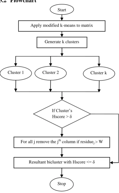
Flowchart

Figure 1. Flowchart of the proposed algorithm

3.3

Algorithm

Input: E(I, J), a gene expression matrix δ, maximal mean squared residue score Output: Resultant bicluster

Phase I: Generate clusters using modified k-means algorithm 1. initialize the centroids, k = 1 to K

2. for i = 1 to K

3. for j = 1 to J 4. read Cij

5. repeat

// create k clusters 6. for e = 1 to I

7. If dist(Ee , Cij) ≤ min_dist , assign Ee to a

cluster

8. recompute the centroid for each cluster until there is no change in the centroids 9. Goto Phase II if cluster’s Hscore > δ 10. else biclusters are generated as output Phase II :

1. For each cluster 2. for i = 1 to I 3. for j = 1 to J 4. compute

Rj= 5. If Rj > W

remove the jth column 6. end for

7. end for

8. If Hscore ≤ δ, biclusters are generated as output 9. else no biclusters are generated as output.

3.4

Time Complexity

In the first phase, a set of k biclusters are generated. Thus the time complexity of Phase I is O(nlk) where n is the total number of objects in the dataset, k is the required number of biclusters identified and l is the total number of iterations, k≤n, l≤n. Since n is the total number of conditions in the gene expression matrix, the Hscore in Phase II can be calculated in O(nk) time. Hence in the worst case the algorithm requires O(lk+nlk) time.

4.

EXPERIMENTAL RESULTS

4.1

Overview of the dataset

Experiments are conducted on the yeast Saccharomyces cerevisiae cell cycle expression data from Cho et al., 1998 [9] in order to evaluate the quality of the proposed algorithm. This dataset has been used in previous biclustering [10], [7] and clustering studies [11]. It is a collection of 2884 genes and 17 experimental conditions, having 34 null entries with -1 indicating the missing values. All entries are integers in the range 0 to 595.

4.2

Bicluster plots for yeast dataset

Figure 2 shows six of the biclusters that we have obtained from the proposed algorithm on Yeast dataset. Some of the biclusters contain all 17 conditions and some contains less than 17 conditions. All the biclusters show similar up-regulation and down-up-regulation. From the visual inspection of Apply modified k-means to matrix

Generate k clusters

Cluster1 Cluster 2

_…..

.

If Cluster’s Hscore > δ

For all j remove the jth column if residuej > W

Resultant bicluster with Hscore <= δ

9 Figure 2. Biclusters extracted from yeast gene expression

data. The biclusters are labeled as (a), (b), (c), (d), (e), (f).

4.3

Performance Comparison

In the Table 1, the average numbers of genes and conditions, average size, average mean squared residue is compared for the proposed algorithm with different distance measures. It is seen that the biclusters produced using the new distance measure as the similarity measure are larger.

Table 1. Comparative study on yeast dataset with different similarity measures

Similarity measures

Bicluster produced

Avg residue

Avg size

Avg gene

Avg condition

Eucledian 235.61

353.2 19.57

16

New_distance 280.28 973.66

60.75

15.75

4.4

Statistical and Biological significance

evolution

The statistical significance of the biclusters obtained is evaluated by calculating the p-values, which signify how well they match with the known gene annotation. The yeast genome gene ontology term finder, GOTermFinder [12], is a tool available in the Saccharomyces Genome Database (SGD) to evaluate the bicluster’s biological significance in terms of associated biological process, molecular functions and cellular components respectively on each discovered biclusters.

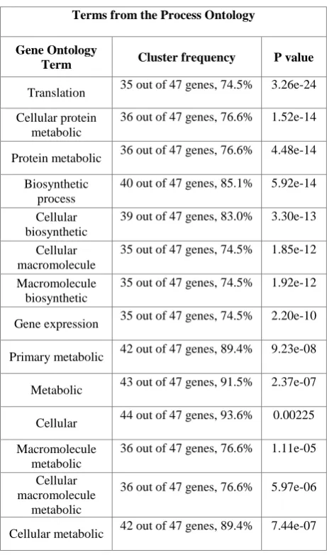
Table 2. Top GO terms from the Process Ontology for biclusters labeled as (a) in Figure 2

Terms from the Process Ontology

Gene Ontology

Term Cluster frequency P value

Translation 35 out of 47 genes, 74.5% 3.26e-24 Cellular protein

metabolic

36 out of 47 genes, 76.6% 1.52e-14

Protein metabolic 36 out of 47 genes, 76.6% 4.48e-14 Biosynthetic

process

40 out of 47 genes, 85.1% 5.92e-14

Cellular biosynthetic

39 out of 47 genes, 83.0% 3.30e-13

Cellular macromolecule

35 out of 47 genes, 74.5% 1.85e-12

Macromolecule biosynthetic

35 out of 47 genes, 74.5% 1.92e-12

Gene expression 35 out of 47 genes, 74.5% 2.20e-10

Primary metabolic 42 out of 47 genes, 89.4% 9.23e-08

Metabolic 43 out of 47 genes, 91.5% 2.37e-07

Cellular 44 out of 47 genes, 93.6% 0.00225 Macromolecule

metabolic

36 out of 47 genes, 76.6% 1.11e-05

Cellular macromolecule

metabolic

36 out of 47 genes, 76.6% 5.97e-06

In Table 2, for example the genes RPL 32, RPL35A, SSB1, RPS11A, RPP2B, RPL37B, RPS26B, RPS21B, RPS22A, RPL43B, RPS5, TMA19, RPS27A, RPL17A, RPS21A, RPL40B, RPL10, STM1, RPS31, RPL37A, RPL38, RPS25B, RPL31B, RPS18B, ASC1, RPS16A, RPS10B, RPP2A, RPS15, CDC33, RPL33B, RPL20B, RPL43A, RPL11A i.e. a total of 35 out of 47 are together involved in the translation process and their statistical significance is 3.26e-24 i.e. p-value. From the table it is clear that the bicluster (a) extracted is distinct along each category. This shows that the biclustering technique produces biologically relevant results.

5.

CONCLUSION

In this paper a new algorithm is introduced which is divided in two phases. In Phase I a modified version of k means algorithm is used where k clusters are generated and the Hscore of each cluster is calculated. If the Hscore of the clusters are greater than the threshold value, then the second phase of the algorithm is implemented where the columns are removed using the residue score of Cheng and Church. The experimental results performed on yeast dataset show that the algorithm is successful in finding biclusters. Also the corresponding plots reveal that the algorithm finds better biclusters because the biclusters show similar up-regulation and down-regulation. Later when a comparison is performed on different similarity measures, it is seen that the new_distance measure produces larger biclusters in comparison to the Euclidian distance measure.

6.

REFERENCES

[1] Shyama Das, Sumam and Mary Idicula, “ Application of Greedy Randomized Adaptive Search Procedure to the Biclustering of Gene Expression Data ”, International Journal of Computer Applications, Volume 2 – No. 3, pp. 0975-8887, 2010.

[2] S. C. Madeira and A. L. Oliveira, “Biclustering Algorithms for Biological Data Analysis: A Survey”, IEEE/ACM Transactions on Computational Biology and Bioinformatics, 1, 24-45, 2004.

[3] Doruk Bozdag, Ashwin S. Kumar and Umit V. Catalyurek, Comparative Analysis of Biclustering Algorithms, 2010.

[4] S. Bergmann, J. Ihmels, N. Barkai, “Iterative Signature Algorithm for the Analysis of Large-scale Gene Expression Data”, Phys Rev E Stat Nonlin SoftMatter Phys, 67(3), 031902, 2003.

[5] A. Prelic, S. Bleuler, P. Zimmerman and E. Zitzler, “A Systematic Comparison and Evaluation of Biclustering Methods for Gene Expression Data”, Bioinformatics 22(9), 1122-1129, 2006.

[6] J. A. Hartigan, “Clustering Algorithms”, New York: John Willey and Sons, Inc, 1975.

[7] A. Tanay, R. Sharan and R. Shamir, “Discovering Statistically Significant Biclusters in Gene Expression Data, Bioinformatics”, 18, 136S-144, 2002.

[8] Y. Cheng and G. Church, “Biclustering of Expression Data”, “Int’l Conf.” on Intelligent Systems for Molecular Biology, 93-103, 2000.

[9] S. Busygin, G. jacobsen, and E. Kramer, “Double Conjugated Clustering Applied to Leukemia Microarray Data” Proc. Second SIAM Int’l Conf. Data Mining, Workshop Clustering High Dimensional Data, 2002. [10] A. Ben-Dor, B. Chor, R. Karp, and Z. Yakhini,

“Discovering Local Structure in Gene Expression Data: The Order-Preserving Sub-Matrix Problem”, Proc. Of the 6th Ann. Int’l Conf on Computational Biology, 1-58113-498-3, 49-57,2002.

[11] L. Lazzeroni and A. Owen, “Plaid Models for Gene Expression Data”, technical report, Stanford Univ., 2000. [12] SGD GO Termfinder