Testing for a common latent variable in a linear regression

Munich Personal RePEc Archive

Testing for a common latent variable in a

linear regression

Wittenberg, Martin

School of Economics, University of Cape Town

31 March 2007

Testing for a common latent variable in a linear

regression

∗

Martin Wittenberg

School of Economics

University of Cape Town

This version March 2007

Abstract

We present a test of the hypothesis that a subset of the regressors are all proxying for the same latent variable. This issue will be of interest in cases where there are several correlated measures of elusive concepts such as misgovernance or corruption; in analyses where key variables such as income are not measured at all and one is forced to rely on various proxies; and where the key regressors are badly measured and one is trying to extract a stronger signal from the regression by adding additional proxies as suggested by Lubotsky and Wittenberg (2006).

We apply this test in three contexts, each characterised by a different estimation challenge arising from data limitations. We reexamine Mauro’s (1995) use of three institutional quality measures in his study of corruption and growth. Here several variables, each potentially measured with error, may all be proxies for a single factor: the quality of governance. Our test suggests that the latent variable is driven primarily by the “red tape” measure, rather than the “corruption” variable on which Mauro focuses.

∗_{I thank Rob Garlick, Murray Leibbrandt, Duncan Thomas, Chris Udry and participants at an African}

Secondly, we look at the correlates of body mass among black South African women. The key variable of interest, namely “wealth” is not measured at all. Consequently we construct an index from a series of asset variables as suggested by Filmer and Pritchett (2001). Our test shows that some assets have independent impacts on the dependent variable. Once this is recognised the “asset index” comes apart.

Finally we analyse the determinants of sleep among young South Africans. The income variable in the survey is badly measured and we supplement it with asset proxies. The test again suggests that some assets are not proxying for the badly measured income variable. We can nevertheless get a substantially stronger signal on the income variable.

Keywords: measurement error, proxy variables, specification test, asset index JEL codes: C12, C13, C52

1

Introduction

In many applied contexts the underlying theory is not strong enough to pin down the precise

form of a regression model. Finding a reasonable specification in these circumstances is likely

to be a somewhat haphazard enterprise. One common problem is that there may be several

candidate measures of the core concepts of the theory. In other cases these may not be

measured at all, or measured extremely badly, and the researcher is forced to rely on proxy

variables. The theory may also be vague on the role of potential covariates.

The textbook treatment of specification error provides an initial assessment of the

im-pact of these problems. In the most benign case, that of adding an irrelevant regressor,

misspecification leads to a loss of efficiency. In other cases, such as the omission of a relevant

variable or choice of incorrect functional form, the result of misspecification is inconsistency

of the estimates. Given these asymmetric costs, researchers are tempted to include

addi-tional covariates to better isolate the impact of the variables of interest. If these addiaddi-tional

regressors do not belong in the “structural” relationship, their coefficients should be

statisti-cally insignificant. Nevertheless in a recent article Lubotsky and Wittenberg (2006) suggest

multiple regression if they are all subject to measurement error. Indeed, they suggest that

deliberately misspecifying the regression by including all available proxies will, in general,

be preferable to creating a summary variable from the available proxies. They provide a

method by which a lower bound on the structural coefficient can be estimated from the

misspecified regression. We summarise the main points of their paper in the appendix. The

validity of the Lubotsky-Wittenberg (LW) estimation procedure hinges, of course, on the

question whether it is plausible that these regressors are, indeed, all functioning as proxies

for the same latent variable.

In this paper we develop a test of the hypothesis that several regressors are acting as

proxies for a single latent variable. This question is likely to be interesting in several different

contexts:

1.1

The role of institutions in economic performance

The importance of institutions for economic performance has become increasingly recognised.

Indeed, institutions seem to make a significant difference in cross-country growth regressions

(Acemoglu, Johnson and Robinson 2001, Bosworth and Collins 2003). Nevertheless many

of the institutional measures are correlated with each other, so that it is difficult to know

whether a particular variable is important in itself or is proxying for some other factor

(Fedderke and Klitgaard 1998). Indeed, Bosworth and Collins (2003) note that a variable

as important as education becomes insignificant in a regression context once one includes a

measure of institutional quality.

Furthermore in many cases there are multiple plausible indicators of the particular

insti-tution that is being measured. In these cases authors have to plump for one or another, or

find some way of combining them. In a frequently cited study, Mauro (1995) had a choice of three different indicators of corruption and misgovernance. He chose to average his

indica-tors. Fundamental to this procedure is the judgement that these indicators are all proxying

for the same underlying latent variable. It may, however, be the case that these institutional

quality variables are themselves only proxying for the effect of some other variable, e.g. the

In this paper we will re-examine Mauro’s conclusions. Our test confirms that these three

observables capture the same underlying variable and that they have a separate impact in

the regression. However, the latent variable is driven primarily by the “red tape” measure,

rather than the “corruption” variable on which Mauro focuses.

1.2

Estimation of “wealth e

ff

ects” through asset variables

There are many data sets in which income or expenditure data is missing, but information

is available on household assets. In an influential paper, Filmer and Pritchett (2001) suggest

that thefirst principal component of the asset variables can be used as a proxy for household

wealth. This method has led to a small growth industry in the analysis of the Demographic

and Health Surveys and, indeed, many other data sets.

In applying this method one would like to know whether the assets do, in fact, proxy for

a common latent variable. Is it possible that any of the assets have an independent effect

on the outcome variable? If so, this would contaminate the interpretation of the index. It

is, after all, a linear combination of the proxies.

We show below that this concern is well-founded. We examine the relationship between

the Body Mass Index and such an asset index in the case of the South African Demographic

and Health Survey. Obesity is becoming recognised as an important health risk among black

South African women, with 22% of all these women being obese. Understanding the economic

and social processes underpinning this trend would be important. The asset index is strongly

positively correlated with the body mass of black South African women. Nevertheless several

of the assets do not proxy only for income. Ownership of a car (unsurprisingly) has a strong

positive impact on body mass. Similarly television ownership has a direct impact. Indeed

after all the assets that do not proxy only for “wealth” are stripped out, the remaining

“wealth” effect is reduced by three-quarters and is significant only at the 10% level on a

1.3

Improving on a badly measured income variable

Generally speaking asset variables have been used in cases where expenditure or income data

is completely unavailable. The Lubotsky and Wittenberg (2006) (LW) estimation procedure

can be used, however, to correct for a badly measured income variable also. It would stand

to reason that augmenting the information from income with that obtained from the asset

variables should improve the estimate. Indeed Szalontai (2006) uses the LW procedure in

precisely this way and shows that the coefficient on the badly measured income variable

almost doubles. As our comments on the asset proxies should highlight, this procedure is

valid only if the assets do not have independent effects.

We reexamine Szalontai’s example, the relationship between sleep and income in South

Africa’s time use survey. Instead of focussing on adults, however, we examine the relationship

among children. We find the same marked increase in the size of the income coefficient.

Nevertheless we alsofind that access to electricity seems to have an independent impact on

sleep times. Ignoring this would lead to an overly high estimate by the LW procedure.

In all three cases having access to a test for a common latent variable changes the

em-pirical analysis. We wish to emphasize that the three cases represent different uses of the

procedure:

• In the first case there are many correlated measures each of which could plausibly feature in the structural equation. In the absence of the test any decisions about how

to summarise the variables, which ones to include and which to leave out, is somewhat

ad-hoc.

• In the second case the concept of interest (income or wealth) is well-defined but is represented by a summary measure extracted from a set of proxies. Our test examines

whether the main regression is correctly specified or whether some of the proxies belong

in it, in which case the coefficient on the “asset index” is misleading.

• The final example deals with a case in which the regression equation is deliberately misspecified in order to counteract attenuation bias on a badly measured variable which

valid or not. In the process of developing this test we also introduce a more efficient

version of the LW estimator.

The plan of the discussion is as follows. In the next section we introduce the central

insight of this paper: that the estimator ofρ, the coefficient on the latent variable in the LW

framework, can best be thought of as a particular type of instrumental variable estimator. If

there are covariates in the model it transpires that more instruments may become available.

This in turn opens up the possibility of testing the validity of the moment conditions. We

introduce this in section 3. First we show how the proxies can be tested individually and

then, in sections 4 and 5 we do so for the system as a whole. This test of the overidentifying

restrictions can be thought of as an omnibus test for all sorts of failures of the model.

Acceptance of the null hypothesis, i.e. of model validity, is equivalent to accepting that the

variables tested are all proxying for a common latent variable.

In section 6 we demonstrate the procedures by means of the three empirical examples.

Section 7 concludes.

2

The regression with proxy variables and one

covari-ate

Let us consider the model

y=xβ+zγ+ε

where we assume thatz is measured accurately andcov(x, z) =σxz is non-zero. We assume

that we have two proxy variables

x0 = x+u0

x1 = xρ1+u1

where we assume that the error variablesuj are uncorrelated withx,z andε. The estimated model is

We have selected a different symbol for the coefficient ofz to indicate that typically this will

not be (not even asymptotically) equal to γ.

As it stands there are no intercepts in this model. We have implicitly projected all

variables on a constant, i.e. we are writing the model in deviations form. This means that

all the errors will automatically have zero mean, so that E¡uju0

j ¢

= σ2

jIn. Hence we can

write the model either in terms of covariances or the expected values of products.

The empirical information at our disposal is summarised in the following correlation

matrix:

⎡ ⎢ ⎢ ⎢ ⎢ ⎢ ⎢ ⎣

β2σ2

x+ 2βγσxz +γ2σz2+σ2ε βσ2x+γσxz βρ1σ2x+γρ1σxz βσxz +γσ2z

σ2

x+σ20 ρ1σ2x+σ01 σxz

ρ2

1σ2x+σ21 ρ1σxz

σ2

z

⎤ ⎥ ⎥ ⎥ ⎥ ⎥ ⎥ ⎦

We observe thatρ1is nowoverdetermined: ρ1 =cov(y, x1)/cov(y, x0)andρ1 =cov(z, x1)/cov(z, x0) This raises the question as to how to estimateρ₁ most efficiently.

Consideration of the form of the GMM estimates of ρ1 given above, suggest that it can be thought of as an instrumental variables estimator in the regression ofx1 on x0. We have

x1 = xρ1+u1

= (x0−u0)ρ1+u1

= x0ρ1+υ1

Note that this cannot be estimated consistently by OLS, since x0 is correlated with u0 and

hence υ1. Since we have assumed that cov(y, x1) = 06 , and cov(y,υ1) = 0 (i.e. neither of the measurement error terms are correlated with any of the terms in the main regression),

y is a legitimate instrument for x1 in this regression. This may seem somewhat surprising

given thaty is actually the dependent variable in a regression in whichx1 is an explanatory

variable. In addition note that if cov(z, x1)6= 0 andz is uncorrelated with any of the error terms, then z is also a legitimate instrument. This suggests that the optimal estimation

What happens if z is correlated with any of theuj terms? In that case it would clearly

be invalid to usez as an instrument. Note, however, that we can write

x1 =x0ρ1+zφ1 +υ1 (1) where by construction υ1 is now uncorrelated with z. We can estimate ρ1 and φ1 in the standard way, using y as an instrument for x0 and z as an instrument for itself. The

estimate of ρ₁ obtained in this way is numerically identical to the “covariate adjusted” estimator suggested in Lubotsky and Wittenberg (2006), except that we do not have to

obtain the residualsfirst.

One advantage of writing the proxy in the form of equation 1 is that it is possible to use

the estimate of φ₁ to calculate a LW estimate of γ similar to the LW estimate ofβ. In this case the proxy variable adjusted estimate would be

b

γ =bθ+bφ₁bb1

Although z is not mismeasured, the fact that b1 is asymptotically nonzero due to the

mea-surement error inxrequires this LW adjustment to be made. With the adjustment, however,

the overall bias in the estimate of γ would be lower than in any regression with some other linear function of x0 and x1, in particular a regression in which only x0 is used as an

ex-planatory variable. This follows, by extension, from the results in Lubotsky and Wittenberg

(2006).

3

Estimation and testing of

ρ

and

φ

proxy by proxy

We will now consider the more general model

y = xβ+Zγ+ε (2a)

x0 = x+u0 (2b)

x1 = xρ1+Z(1)φ1+u1 (2c)

· · ·

where cov(ε, uj) = 0. Furthermore we assume thatE(Z0_u

0) =0. Since Z is assumed to contain a column of ones this implies thatu0 has mean zero. Consequentlyx0 is an instance

of “classical measurement error”. If this assumption is violated, the LW procedure can still

be applied, but the coefficients of the Z variables that are correlated with u0 will not be

correctable by means of the procedure outlined below. We allow the other k proxies for x,

viz. x1, . . . , xkto be moreflexibly defined. In particular we suppose that the deviations from

the latent variablex may be systematic and explicable in terms of some of the covariates.

We assume that the matrix of covariates Z can be partitioned as

Z =h Z(i) Z−(i)

i

into variables Z(i) that have a direct effect on the proxy xi, when controlling for the latent

variable x, as well as variablesZ₋(i) that are correlated withxi only throughx. If there is a

variable that is orthogonal tox andxi we will include it inZ(i) to remove any ambiguity. It

will generally be the case that Z(i) will contain at least a column of ones for the intercept.

With constants in all equations we can assume that all error terms are mean zero. Finally

we assume that Z₋(i) is also non-empty. Note that in many applications including the ones

reported on below we may be able to partition the matrix in the same way for every proxy.

With these assumptions, we can write the i-th proxy as

xi = x0ρi+Z(i)φi+ui−u0ρi

= M(i)δi+υi (3)

where M(i) =

h

x0 Z(i)

i

and δi =

⎡ ⎣ ρi

φi

⎤

⎦. Furthermore by our assumptions,

Z0¡_xi−x

0ρi−Z(i)φi ¢

= 0 (4a)

y0¡_xi−x

0ρi−Z(i)φi ¢

= 0 (4b)

and hence ρi and the coefficient vector φi can be consistently estimated by instrumental

An appropriate estimator for this equation would therefore be the generalised IV estimator,

or two-stage least squares estimator

bδi = ³

M0

(i)Zy

¡ Z0

yZy ¢−1

Z0

yM(i)

´−1

M0

(i)Zy

¡ Z0

yZy ¢−1

Z0

yxi (5)

where Zy is the matrix of instruments, i.e.

Zy =h y Z i

(6)

With these estimates for ρi andφi the LW estimates ofβ and γ will be given by b

β = b0+

k X

i=1

b

ρibi (7a)

b

γj = bθj + k X

i=1

b

φijbi (7b)

wherebθj is the unadjusted coefficient onzj in the multiple regression with all the proxies

included and where bφ_ij = 0 if zj _∈/Z(i).

If Z₋(i) is non-empty it is possible to test for the validity of the LW model by means of

a test of the overidentifying restrictions. A particularly easy form of such a test is described

in Davidson and MacKinnon (1993, p.236). They show thatntimes the uncentered R2 _from

a regression of the IV residuals on the instruments Z is distributed as χ2 _{with degrees of} freedom equal to the degree of overidentification. In this case the degree of overidentification

is exactly equal to the number of variables inZ₋₍i).

The null hypothesis for this test is that the moment conditions in equations 4 are all

valid. This hypothesis could be rejected for a number of reasons:

1. ε is correlated with any of the ui terms

2. one or more of the covariates in Z₋(i) is correlated with any of the ui terms

3. The proxy model is misspecified, i.e. it is not the case that

This could be due to either the fact that it is not the case that

xi =xρ_i+Z(i)φi+ui

or that it is not the case that

x0 =x+u0

4. The main regression model is misspecified

Most of these would be reasons for being sceptical about the validity of applying the LW

model. If the test fails for the second reason, however, it would be possible to re-partition

the covariates and include the offending variables in the controls Z(i). If all covariates end

up being included it is, of course, no longer possible to test the model. This may also be an

indication that the LW model is of dubious value.

As an aside, we note that the “covariates adjusted” estimator ofρsuggested in Lubotsky and Wittenberg (2006) is identical to the estimate obtained if Z(i) = Z, i.e. if none of

the covariates was a legitimate instrument. We would expect therefore that the procedure

outlined above should lead to more efficient estimates than that given in the original paper.

4

Systems estimation of

ρ

and

φ

According to the model given in equations 2 there arek equations of the type 3 to estimate.

We can “stack” these equations in the standard way: ⎡ ⎢ ⎢ ⎢ ⎢ ⎢ ⎢ ⎣ x1 x2 ... xk ⎤ ⎥ ⎥ ⎥ ⎥ ⎥ ⎥ ⎦ = ⎡ ⎢ ⎢ ⎢ ⎢ ⎢ ⎢ ⎣

M(1) 0 · · · 0

0 M(2) · · · 0 ... ... . .. ...

0 0 · · · M(k) ⎤ ⎥ ⎥ ⎥ ⎥ ⎥ ⎥ ⎦ ⎡ ⎢ ⎢ ⎢ ⎢ ⎢ ⎢ ⎣ δ1 δ2 ... δk ⎤ ⎥ ⎥ ⎥ ⎥ ⎥ ⎥ ⎦ + ⎡ ⎢ ⎢ ⎢ ⎢ ⎢ ⎢ ⎣ υ1 υ2 ... υk ⎤ ⎥ ⎥ ⎥ ⎥ ⎥ ⎥ ⎦ (8)

x_{v =} M_{δ+υv (9)}

In the special case where the same control variablesZ(i)=Zu are used in every equation the

matrix M _{takes on the particularly simple form}

M _{= Ik⊗}

h

x0 Zu

i

where Mx =h x0 Zu

i

.

The systems version of the proxy by proxy estimation outlined above would be to define

the matrix of instruments

Z_{v =}

⎡ ⎢ ⎢ ⎢ ⎢ ⎢ ⎢ ⎣

Zy 0 · · · 0 0 Zy · · · 0

... ... ... ...

0 0 · · · Zy

⎤ ⎥ ⎥ ⎥ ⎥ ⎥ ⎥ ⎦

= Ik_⊗Zy (11)

and then define the “2SLS” estimator

b

δ2SLS = ³

M0Z_v(Z0_vZ_v)−1Z0_vM´−1M0Z_v(Z0_vZ_v)−1Z0_vx_{v (12)}

which is numerically equal to the proxy by proxy estimation ofδ given in equation 5. This estimator, however, may not be efficient, since the covariance matrix of υv is not

diagonal. It is obvious that the vectorυi and the vectorυj are correlated. In fact a typical

co-variance between an element ofυiandυj will be given bycov(υi,υj) =cov ¡

ui−u0ρi, uj−u0ρj ¢

=

σij−ρjσ0i−ρiσ0j +ρiρjσ20. Let us denote this as υij. Then E(υvυ0v) = Ψ

= Σ⊗In

where Σ= ⎡ ⎢ ⎢ ⎢ ⎢ ⎢ ⎢ ⎣

υ11 υ12 · · · υ1k

υ12 υ22 · · · υ2k

... ... ... ...

υ1k υ2k · · · υkk

⎤ ⎥ ⎥ ⎥ ⎥ ⎥ ⎥ ⎦

This suggests that the system of proxy equations could be more efficiently estimated as a

system, taking these cross-equation correlations into account.

A brief consideration of the formal properties of the model shows that the GLS estimator

(Davidson and MacKinnon 1993, Mittelhammer, Judge and Miller 2000). This means that

estimation of δ and hence ρ can proceed with readily available software. Furthermore the asymptotic properties of this estimator are well established.

Nevertheless it is useful to briefly go through the derivation of the estimator, since we will

use some of the intermediate results in section 5. We follow the treatment in Mittelhammer

et al. (2000, pp.462—465) and develop the estimator as the optimal GMM estimator from the

population moment condition

E(Z0_v(x_v−M_{δ)) =}0 ₍₁₃₎

This yields the sample counterpart

1

nZ

0

v(xv−Mδ) =0

and hence the GMM estimator

b

δ(W_{) = [}M0Z_vWZ0_vM_]−1M0Z_vWZ0_vx_{v (14)}

for some positive definite weighting matrix W_{. Indeed with} W _{= (}Z0

vZv)−1 we get the

“2SLS” estimator of equation 12. The optimal weighting matrix, however, is

w−_∗1 = cov³n−12Z0_vυ_v

´

= n−1E(Z0

vυvυ0vZv)

= n−1E¡(Ik⊗Zy)0(Σ⊗In) (Ik⊗Zy)¢

= Σ⊗E¡n−1Z0

yZy ¢

(15)

W _{is therefore proportional to Σ}−1 _⊗¡_Z0

yZy ¢−1

and the corresponding GMM estimator is

given by

δGM M = h

M0³_Σ−1

⊗Zy¡Z0

yZy ¢−1

Z0

y ´

Mi−1M0³_Σ−1

⊗Zy¡Z0

yZy ¢−1

Z0

y ´

x_{v (16)}

The matrix Σ is unknown, but can be consistently estimated using the residuals from any

consistent GMM estimator. The 2SLS estimator (12) is particularly convenient in this regard.

We have

b

Σij =

1

nbυ

0

whereυ_bi andbυj are the vectors of residuals from thei-th andj-th proxy estimation

respec-tively. Using this in place of Σgives the estimated weighting matrix

c

W_=Σb−1 _⊗¡_Z0

yZy ¢−1

(17)

and correspondingly the estimated optimal GMM estimator bδGM M or three-stage least

squares estimator.

In the case where the same control variables Z(i) = Zu are used in every equation, we

can substitute equation 10 into equation 16. This yields

b

δGM M = h

b

Σ−1_⊗M0

xZy ¡

Z0

yZy ¢−1

Z0

yMx i−1h

b

Σ−1_⊗M0

xZy ¡

Z0

yZy ¢−1

Z0 y i x_v = ½

Ik_⊗³M0

xZy ¡

Z0

yZy ¢−1

Z0 yMx ´−1 M0 xZy ¡ Z0 yZy ¢−1

Z0

y ¾

x_{v (18)}

This, however, is numerically identical to the proxy by proxy estimation ofδ by 2SLS! This

finding parallels the result that least squares estimation and GLS estimation of a SUR system

with identicalX matrices are equal (see for instance Mittelhammer et al. 2000, p.453).

5

Speci

_fi

cation testing

Just as it is possible to test the overidentifying restrictions proxy by proxy, it is possible to

do so on the system as a whole. The appropriate test statistic in this case will be given by

h

Z0

v ³

x_v−Mb_{δGM M}´i0WchZ0

v ³

x_v−Mb_{δGM M}´i_→d _χ2_(d)

(Mittelhammer et al. 2000, pp.438—9) whereWc _{is given by equation 17 and d is the degree}

of overidentification, i.e. the number of instruments used in the system as a whole minus

the number of moment equations. The test statistic τ can be simplified to

b

υ0v ³

b

Σ−1⊗Zy¡Z0

yZy ¢−1

Z0

y ´

b

υv

where _bυv is the vector of stacked IV residuals. Now note that this is equivalent to b

υ0_v³Ik⊗Zy¡Z0

yZy ¢−1

Z0

y ´0³

b

Σ−1⊗In´ ³Ik⊗Zy¡Z0

yZy ¢−1

Z0

y ´

b

Let

bb

υ=³Ik_⊗Zy¡Z0

yZy ¢−1

Z0

y ´

b

υv

This is the vector of fitted values from the artificial regression of the residuals bυv on the

matrix of instrumentsZ_{v. Hence the test statistic can also be written as}

bb

υ0³Σb−1⊗In´bbυ

In the trivial case where this estimator is applied to a “system” of only one equation Σb−1 ₌

b

σ−2and the test statistic is identical tonR2

u in the regression ofbυv onZv. WheneverΣb−1⊗In

isnotequal toσ_b−2Ikn, however, this statistic will not be computable in this manner. Instead, let

b

Σ−1 =

⎡ ⎢ ⎢ ⎢ ⎢ ⎢ ⎢ ⎣

α11 α12 · · · α1k

α21 α22 · · · α2k

... ... ... ...

αk1 αk2 · · · αkk

⎤ ⎥ ⎥ ⎥ ⎥ ⎥ ⎥ ⎦

and let bbυi refer (in the obvious way) to the vector of fitted values corresponding to the i-th

proxy then

bb

υ0³Σb−1_⊗In´bbυ = h bbυ0₁ bbυ0₂ · · · bbυ0_k

i ⎡ ⎢ ⎢ ⎢ ⎢ ⎢ ⎢ ⎣

α11In α12In · · · α1kIn

α21In α22In · · · α2kIn ... ... . .. ...

αk1In αk2In · · · αkkIn ⎤ ⎥ ⎥ ⎥ ⎥ ⎥ ⎥ ⎦ ⎡ ⎢ ⎢ ⎢ ⎢ ⎢ ⎢ ⎣ bb υ1 bb υ2 ... bb υk ⎤ ⎥ ⎥ ⎥ ⎥ ⎥ ⎥ ⎦

= h Pk_i=1αi1bbυ

0

i Pk

i=1αi2bbυ

0

i · · · Pk

i=1αikbbυ

0 i i ⎡ ⎢ ⎢ ⎢ ⎢ ⎢ ⎢ ⎣ bb υ1 bb υ2 ... bb υk ⎤ ⎥ ⎥ ⎥ ⎥ ⎥ ⎥ ⎦ = k X i=1 k X j=1

αijbbυ

0

ibbυj (19)

If we define the matrixB as

and we note that B is symmetric, it is easy to see that

k X

i=1

k X

j=1

αijbbυ

0

ibbυj =tr ³

b

Σ−1B´

If the artificial regression fits perfectly, so that bbυj =bυj, then B =nΣb and the test statistic

will be kn.

The important point to note is that the calculation of the test statistic does not require

the formation of any kn×kn matrices. Indeed provided that one uses the same partition of the Z matrix in each proxy equation there is no need to compute anything other than

the proxy-by-proxy two stage least squares estimates and the residuals from them. Even in

this case one may want to utilise three stage least squares routines since these conveniently

calculate the matrixΣb. Certainly one will need to do so if one wanted to test restrictions on

theρ vector.

In the case where the same controls are used in each proxy equation it is easy to calculate

the degrees of freedom for the hypothesis test. If we let the number of variables that arenot

in Zu be l, i.e.

l=rank(Z)₋rank(Zu)

then the degrees of freedom for the test will be d = lk, i.e. the number of instruments

(rank(Z) + 1)k used less the number of moment equations, i.e. (1 +rank(Zu))k.

The null hypothesis for this test is that the moment condition given in equation 13 holds. As we noted above, a rejection of the null can occur for a number of different reasons:

• A correlation between ε and any of the ui terms. In this case y would cease to be an appropriate instrument. This implies that the proxy variable xi is not proxying only

for the latent variable x, but should be in the main regression.

• A correlation between any of the zj variables used as instruments and any of the ui

terms. In this case zj should be treated as a control in equation i and not as an

instrument.

• A misspecification of the main regression

In short rejection of the null hypothesis should probably be taken as evidence that the

model should be seriously rethought, although it may be technically possible to respecify it

in ways that provide consistent estimates ofρ.

In our empirical applications we view rejection of the model as a sign that the model

is inadequate. For instance, in the “corruption” example we will see that the system test

rejects the assumption that the three “institutional” variables are proxying for secondary

school enrolment.

In the case of the “asset index” example we have to be somewhat more circumspect,

because it is clear by considering the nature of the variables involved that some of the other

covariates should be treated as controls and not as instruments. Nevertheless even once that

correlation is acknowledged the system test still rejects the idea that all the assets are simply

proxying for a commmon latent variable (“wealth”). We interpret this as evidence that some

of the assets belong in the main regression.

6

Applications: proxying for institutions, wealth and

income

In order to get a sense how these techniques perform on real data we apply them to three

contexts where we suspect that there may be common latent variables:

1. A cross-country study of the relationship between institutions and investment.

2. A study on a Demographic and Health Survey, where there is no income or expenditure

data, but there are asset proxies

3. A study on a data set where the income variable is measured very badly, but there are

asset proxies

The three examples present some of the spectrum of cases where our specification test

are elusive and difficult to capture. As a result different measures may be available and the

analyst needs to decide whether it is permissible to combine these in some way.

In the second case the variable of interest is not measured at all, but we have a number

of proxies available. The problem is, that some of these may have effects independent of the

latent variable they are supposedly proxying for.

The last example is, perhaps, the cleanest case for the Lubotsky and Wittenberg (2006)

procedure, since there is a ready made proxy to serve as numeraire — the income variable

itself. Here the key issue is whether one can get a measure of the impact of that variable

that is subject to less attenuation bias.

6.1

The link between corruption and investment

Mauro’s study of the link between corruption and growth has been the landmark study in this

area. He suggests that a key link in the chain between corruption and growth is investment —

corruption and bad institutions have the effect of significantly lowering the investment rate.

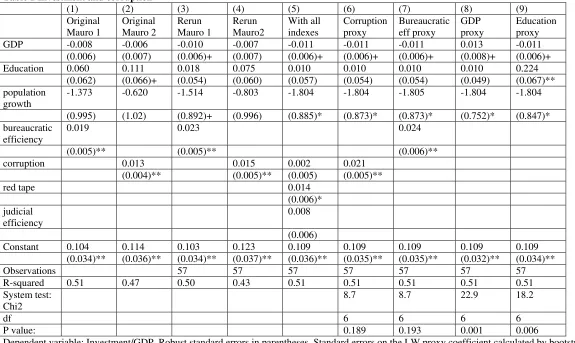
In Table 1 we reexamine the link between corruption and investment using a data set

that is as close as possible to the original. The first two columns of that table reproduce

directly the results from thefirst two columns of Mauro’s Table VI (1995, p.699). We re-run

those regressions with our data set in columns three and four. The coefficients are close to

those reported by Mauro and the significance levels are close as well. The main result is that

the “bureaucratic efficiency” and corruption index both have a direct and statistically highly

significant impact on the level of investment (relative to GDP). We note that high values of

the index correspond to good institutions, so that lower corruption and better efficiency are

associated with higher investment.

In column five we insert all three of the indexes that Mauro considered. Only the “red

tape” index turns out to be significant, although the other two indexes also record positive

coefficients. The reason for this is may simply be that the indexes are all too highly correlated

with each other and subject to too much measurement error. Indeed Mauro’s “bureaucratic

efficiency” index is simply the arithmetic average of the three indexes and is constructed

We test the hypothesis that all three variables are simply proxying for a common latent

variable in column six. We use the “corruption index” as the chief proxy x0, i.e the proxy

that fixes the scale of the latent variable. As the test statistic and p-value at the foot of

that column indicate, the data accept the hypothesis that there is a common latent variable.

We see that the optimal linear combination of the indexes leads to a sizable increase in the

measured coefficient from 0.015 to 0.021, which is around a 40% improvement.

We can calculate the LW index that would correspond to this estimate. It is given by

LW = 0.11 corruption+ 0.66red tape + 0.35 judicial effectiveness

The coefficients do not sum to one, which suggests that although all three variables are theoretically scored on a scale from 1 to 10, the “red tape” and “judicial effectiveness” scores are effectively operating on a more compressed scale than the corruption ones. Indeed

the range and standard deviation of those two variables is somewhat smaller than those of

the corruption index. The main point is that the latent variable that is picked by the data

looks much more like a “red tape” variable than a “corruption” one.

Column seven checks to see whether the “bureaucratic effectiveness” index can be im-proved on. In this regression we are including the bureaucratic effectiveness index as proxy

x0 and also include the “red tape” and “judicial effectiveness” index. In this case the

im-provement brought about by the LW procedure is minor. In short simply averaging the

three indexes goes almost all the way to reducing the attenuation bias in this case. When

compared to the optimal LW index the data, however, again suggest a major role for red

tape. The index in this case is given by

LW = 0.29 bureaucratic efficiency + 0.51red tape + 0.22 judicial effectiveness

Since the bureaucratic efficiency index is the simple average of the corruption, red tape and judicial effectiveness indices, the data again suggest that the optimal weighting of the three

indexes is around 10% of the corruption index, 60% of the red tape one and 30% of the

judicial effectiveness one.

In the last two columns of table 1 we consider whether the three indexes of good

per capita) or education. As theχ2 _{statistics and p-values indicate, the data soundly reject} these hypotheses.

In summary the analyses support Mauro’s decision to combine the three indexes. They

even suggest that averaging them is close to optimal. However the data also make clear that

most of the work in the regression is being done by the “red tape” index. If there is a latent

variable that all three indexes are proxying for, then it looks much more like a “red tape”

one than a corruption one.

6.2

Body mass and asset ownership

There has been a rapid increase in obesity, even in developing countries (Popkin 1999). South

Africans have followed this trend, with many showing high body mass even in otherwise

poverty stricken communities (Case and Deaton 2005). This has led to an increase in the

prevalence of hypertension and strokes in contexts where one might not have expected to

see this (Kahn and Tollman 1999). Understanding the socio-economic correlates of obesity

is therefore of considerable interest.

The main data set available for exploring this relationship is the South African

Demo-graphic and Health Survey. Like other such surveys, it has extensive health information but

very few socio-economic variables. In particular it has no income or expenditure

informa-tion. A standard procedure now in such cases is to estimate an asset index by principal

components (Filmer and Pritchett 2001) and to use this as a proxy for wealth.

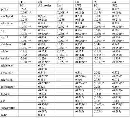
In Table 2 we show a set of regressions in which the body mass of black South African

women is regressed on asset proxies and a set of individual and household attributes. We

focus on women because obesity is particularly prevalent in this group. The dependent

variable is the body mass index (BMI) defined as weight (in kilogram) divided by height

(in metres) squared. The first column shows that a one unit increase (equivalent to a

standard deviation increase) in the asset index is associated with an average increase of

0.599 in the BMI. This translates into an increase of 1.4kg (3 lbs) for a woman of average

height (1.577m). This suggests that women of higher economic status would also be heavier,

disproportionately of low income communities. This finding is reinforced by the strongly

positive coefficient on education.

In column 2 we include the proxies separately while column 3 provides an estimate on

the coefficient of the underlying latent variable if we go on the assumption that all the

assets are proxying for a common latent variable. We have used telephone ownership as

our x0 proxy. Since we would really like an estimate of the impact of expenditure, we

projected telephone ownership on log household expenditure in the South African Income

and Expenditure survey. This led to the estimate

tel=₋2.175 + 0.2585 ln (expenditure)

i.e. _bρ₀ = 0.2585. By rescaling the telephone variable by the reciprocal of 0.2585 it should be on a scale where a one unit increase in the latent variable will correspond to a one

unit increase in log (expenditure). As it is, the standard deviation of the log of household

expenditure happens to be 1.076. The coefficient on the LW index in column 3 should

therefore correspond roughly to a standard deviation increase in log household expenditure.

It should therefore be directly comparable to the coefficient on the asset index. As the theory would suggest, the LW procedure produces a coefficient that is markedly larger.

Nevertheless before jumping to conclusions it would be prudent to test that the asset

variables are, indeed, all proxying for a common latent variable. In order for this test to

pass muster we need to allow for correlations between the “employment” and “education”

variables and the assets. These two variables almost certainly have effects on the

accu-mulation of assets independent of total expenditure (or wealth). Employment is likely to

feature because many household assets (such as television sets) are purchased through loan

agreements and employment makes such acquisitions easier, even controlling for household

wealth. Education is likely to influence asset accumulation both as a taste shifter and as

a necessary input into the utilisation of some assets. It therefore does not make sense to

think of asset ownership being correlated with these two variables only through the latent

variable. The specification test is thus implemented using age, the square of age, household

composition (number of children and number of adults) and being a smoker as exogenous

Strikingly, the specification test roundly rejects this model. The individual specification

tests on six of the assets are particularly vehemently rejected, these being access to electricity,

television, refrigerator, bicycle, car and sheep/cattle ownership. Once these are allowed to

have independent effects (as in column 4 of Table 2), the specification test is happy to

accept that the remaining assets could proxy for a common latent variable. Interestingly

not all of the assets rejected by the specification test turn out to have statistically signficant

coefficients. Whatever they might be measuring, however, it is not the same kind of thing

as what the other assets are capturing. So, for instance, it is quite likely that ownership of

sheep and cattle represents not just wealth, but traditional values and a rural location. To

the extent to which rural diets and lifestyles are lagging behind the shifts that are driving

the obesity epidemic in urban areas, this index may function differently in the regression.

Indeed we observe that the point estimates in columns 2 and 4 are negative.

Two of the assets stand out for their very strong effects. Car ownership is associated

with almost a full unit increase in mean BMI. This represents a 2.4kg (5.3lb) increase for

a woman of average height. Television has an identically strong effect. The specification test rejects the idea that these are merely income, expenditure or wealth effects. They are lifestyle effects which come with the acquisition of those particular assets.

When we put these variables into a multiple regression together with the asset index (in

column 5) we notice that the coefficients are 22% smaller. In the case of car ownership the

variable is significant only at the 10% level. We would therefore make misleading inferences.

Of course one is asking for trouble if one includes assets twice over — in the asset index and

separately in the regression. In column six we therefore recalculate the asset index only

over variables that we do not intend to include separately in the regression. This regression

provides a very similar picture to that given by the LW procedure (in column 4), except that

the coefficient on the asset index is 30% smaller. It is completely insignificant, while the LW

asset index would be significant at the 12% level.

Nevertheless neither regression makes a strong case for an independent and sizable wealth

or income effect. It looks as though improvements in socio-economic status lead to increases

in body mass largely through the more sedentary lifestyle that they help to buy. A simple

6.3

Sleep and income

In the previous cases the latent variable was not measured at all. We now consider an

example where the variable is measured, but badly. The application is the demand for sleep

among school going South Africans. The pioneering study on the economic determinants of

sleep was by Biddle and Hamermesh (1990). They argued that the length of sleep was not

purely biologically determined but responded to economic signals. The opportunity cost of

sleep is the wage foregone and so one would expect high wage earners to sleep less than low

wage ones. They show this with US time use data. Szalontai (2006) examines the same

relationship on South African data and finds similar results. Because his income variable

is badly measured he employs the Lubotsky-Wittenberg procedure using a number of asset

variables to extract a stronger signal. Indeed the coefficient increases by 75% in absolute

value.

We will re-examine this procedure but on a different subsample, viz. school age

chil-dren. A recent study suggested that sleep in this group also strongly decreases with income

(Wittenberg 2005). In this case the opportunity cost of sleep cannot be the wage, so there

must be other explanations, including the entertainment opportunities foregone.

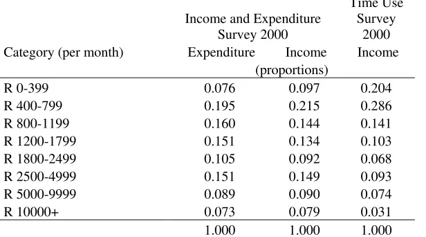
The data for the South African studies comes from the South African time use survey

conducted by Statistics South Africa (Budlender, Chobokoane and Mpetsheni 2001). One of

the problems with investigating economic relationships on this data set is that the income

information is very poor. In this it is not unique: in all surveys there is some trade off

between the breadth of issues covered and the quality of information obtained on particular

variables. Surveys which ask a simple income question and do not extensively probe are

unlikely to get quality income data. The extent of the problem can be seen in Table 3,

which contrasts the total household income distribution from the Time Use Survey and the

expenditure and income distributions from an Income and Expenditure Survey conducted

by Statistics South Africa in the same year, i.e. 2000.

It is clear that total household income in the Time Use Survey has been measured with

considerable error. It also seems clear that this error is not classical measurement error in

so that the measurement error termu0 has a non-zero mean. This means that the intercept

term in the regression will have an additional unknown bias. Furthermore it is plausible that

the scale of the measurement error may be correlated with some of the covariates. The LW

“corrected” coefficients of these terms should therefore be viewed with some caution.

The scale of the underreporting however also increases the attractiveness of the LW

procedure. It seems clear that households with very low reported incomes, but possessing

fridges, stoves and televisions must be better offthan households without those. Including

asset proxies would control for income much better than using the reported income categories

alone.

For the purposes of the regressions we have turned the discrete income categories into

a continuous variable, by taking the midpoints of the categories and twice the lower bound

of the open category. The latter is recommended by Charles Simkins (personal

communica-tion), based on the fact that the income distribution at the top end is roughly Pareto with

parameter just under two. This adds an additional level of noise to the variable which will,

however, be of secondary influence compared to the underreporting shown above.

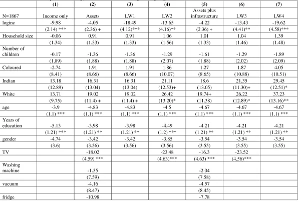
In column 1 of Table 4 we report a simple regression of minutes spent sleeping during an

average night during the school week (Monday to Friday). The sample is restricted only to

individuals who are actually observed attending school in the time diaries. The coefficient on log income is around -10, which would translate to a 35 minute difference between children

with the median income (R600) and the richest children (R20 000). Adding in the proxies we

see a marked drop in this coefficient, but significant coefficients on “fridge” and “TV”. The LW estimates in columns (3) and (4) make different assumptions about which covariates are

correlated with the proxies and which are independent of the measurement errors.

In column (3) we assume that all covariates are exogenous. This is effectively what Szalontai assumed also. The coefficient is 85% larger, but we observe that the specification

test roundly rejects the underlying assumptions. Given South Africa’s history it is unlikely

that the racial dummies will be exogenous. Black South Africans are likely to have an

“asset deficit” which is not simply a function of income. We might assume also that some

of the household composition variables might affect the acquisition of particular types of

survey as exogenous. The individual proxy specification tests now come out as accepting the

null hypothesis, except in the case of television ownership. We have consequently allowed

television ownership to have an independent effect on sleeping times. The LW estimates given in column (4) still show a marked increase on the income coefficient compared to column (1). The point estimate on income corresponds to about 48 minutes difference in

sleep times between the median income and the top. This is a nontrivial impact, particularly

if one bears in mind the additional 23 minutes loss of sleep attendant on owning a television!

As this regression performs well on all the specification tests we might be happy to leave

the issue. There seem to be two factors that matter: income raises the opportunity costs of

sleep, while ownership of a television does so even when controlling for income. This simple

picture is, however, muddied by the results shown in the remaining columns. In column five

we have added in two “infrastructure” proxies - use of electricity for lighting and living in

a brick dwelling. The LW estimates reported in column (6) correspond to the same model

as that accepted by the data in column (4), except that these additional proxies have been

used in the LW procedure. In this case, however, the specification test roundly rejects the

validity of the model. More particularly it suggests that electricity should be in the main

model. It also raises the prospect that perhaps it is not television per se that is important

for sleep, but access to electricity and the attendant opportunities.

In columns six and seven we explore two competing hypotheses:

• In column six we have the hypothesis that only the log of income and television own-ership belong in the structural equation. Access to electricity is interpreted in the LW

model as just another proxy for mismeasured income. As we have noted above, this

model is not supported by the specification tests - either for the “electricity” proxy

equation or for the system as a whole.

• In column seven we explore the hypothesis that only the log of income and access to electricity belong in the structural equation. TV ownership is relegated to the status

of a proxy for income. This model is accepted by the data at conventional levels of

significance despite the fact that the TV ownership proxy has a statistically significant

The procedure that we have employed in adjudicating whether television or electricity

are structural is reminiscent of Granger causality tests. Like those tests it is possible for the

answers to be less clear cut. The data might have suggested that both variables belong in

the main regression or that neither do. Of course tests are hardly ever completely decisive

and the power of the tests may be inadequate.

Reviewing the evidence available in Table 4 we come to the conclusion that a point

estimate of around -18 is probably a reasonable guess at the impact of income on sleep. The

naive LW procedure did not lead to a distorted estimate in this case, although it did not

reveal the additional impact of electricity or TV. The point estimate would correspond to a

difference of about an hour sleep per day between kids at the median income versus children

in the top income bracket. In addition to this children with electrified houses would sleep

24 minutes a day less. One of the opportunities opened up by larger incomes is, of course,

the ability to watch television. So television probably matters - but as an outcome rather

than a structural determinant. Indeed an initial look at patterns of television watching

suggests that television viewing may be related to income in inverse U fashion - increasing

with income and then decreasing at the top. The richest children probably have many more

non-TV opportunities (e.g. internet chat rooms) to while away the nights. In short there are

non-technical reasons for believing that the specification tests have picked out a reasonable

model.

7

Conclusion

In all three empirical applications the ability to test for a common latent variable has added

to our understanding of the underlying relationships. In the case of the institutional quality

scores we could show that it was reasonable to try to combine them. We could also pinpoint

which of the variables were doing most of the work in the regression. This suggested that

the impact being estimated was that of “red tape” more than “corruption”.

In the second example our test really picked the composite index apart. It showed

that some of its components, notably car and television ownership, were having large and

by lifestyle changes.

In the third case the main issue was to estimate the coefficient on log income more

reliably. We showed that a naive application of the Lubotsky-Wittenberg procedure (2006)

would miss the fact that some assets seem to have impacts independent of income. In

particular, access to electricity seems to open up activities (such as television watching) that

crowd out sleep. In this case we also showed that the tests can be used to think about the

“structural” relationship between proxies. We did this by means of a Granger-style “proxy

test”. We tested whether:

• TV could be proxying for income controlling for the presence of electricity or

• Electricity could be proxying for income controlling for the presence of TV.

Ultimately, however, these techniques are no substitute for thinking about the underlying

relationships theoretically. Indeed the LW procedure cannot in any real way substitute

for proper judgement or “fix” bad data. If income is badly measured the LW procedure

provides the promise that one can get an additional measure of people’s control of resources

by taking account of their assets. But this is second prize compared to better quality income

information. Furthermore as these examples should make clear the “fix” needs to be run

with proper caution.

In this paper we have shown how the LW procedure can be run more efficiently. The

empirical results suggest that it can significantly strengthen the estimated coefficients.

Un-der certain circumstances this could make a difference to how one interprets the output.

Nevertheless, before applying it, it would be prudent to run the specification test developed

in this paper.

A

Appendix: The LW procedure

Lubotsky and Wittenberg (2006) analyse the model

y = βx∗ +ε

where ρ₁ = 1 and the errorsuj are uncorrelated withε andx∗ _{and have mean zero, but are} otherwise unrestricted. They show thatρj can be consistently estimated by

ρ_j = cov(y, xj)

cov(y, x1)

They suggest that in general one should include all proxies in the main regression and

aggregate the coefficients up according to the formula:

bρ=bρ0b=

k X

j=1

cov(y, xj)

cov(y, x1)

bj

wherebis the vector of OLS regression coefficients (i.e. bj is the coefficient on thej-th proxy

in that regression). They argue that this will produce a lower bound on the true coefficient

β. Furthermore this lower bound will have less attenuation bias than estimates obtained by any other linear combination of the proxy variables. They also show that this procedure

implicitly constructs an index from the proxies, which can be explicitly calculated as

xρ= 1

bρ

k X

j=1

xjbj

If there are covariates in the model, they suggest that the procedure be run after the effect

of the covariates has been removed by projecting both y and the proxies on the covariates.

References

Acemoglu, Daron, Simon Johnson, and James A. Robinson, “The colonial origins

of comparative development: an empirical investigation,” American Economic Review,

2001, 91 (5), 1369—1401.

Biddle, JeffE. and Daniel S. Hamermesh, “Sleep and the Allocation of Time,”Journal

of Political Economy, 1990, 98 (5 Part 1), 922—943.

Bosworth, Barry P. and Susan M. Collins, “The empirics of growth: An update,”

Budlender, Debbie, Ntebaleng Chobokoane, and Yandiswa Mpetsheni, A Survey

of Time Use: How South African women and men spend their time, Pretoria: Statistics

South Africa, 2001.

Case, Anne and Angus Deaton, “Health and wealth among the poor: India and South

Africa compared,”American Economic Review Papers and Proceedings, 2005.

Davidson, Russell and James G. MacKinnon,Estimation and Inference in

Economet-rics, New York: Oxford University Press, 1993.

Fedderke, Johannes and Robert Klitgaard, “Economic Growth and Social Indicators:

An Exploratory Analysis,” Economic Development and Cultural Change, 1998, 46 (3),

455—489.

Filmer, Deon and Lant H. Pritchett, “Estimating Wealth Effects Without

Expendi-ture Data — Or Tears: An Application to Educational Enrollment in States of India,”

Demography, February 2001,38 (1), 115—132.

Heston, A., R. Summers, and B. Aten, “Penn World Table version 6.2,” September

2006. Center for International Comparisons of Production, Income and Prices,

Univer-sity of Pennsylvania.

Kahn, K. and S.M. Tollman, “Stroke in rural South Africa – contributing to the little

known about a big problem,” South African Journal of Medicine, 1999, 89 (1), 63—65.

Lubotsky, Darren and Martin Wittenberg, “Interpretation of regressions with multiple

proxies,”Review of Economics and Statistics, 2006,88 (3), 549—562.

Mauro, Paolo, “Corruption and Growth,” Quarterly Journal of Economics, 1995,110 (3),

681—712.

Mittelhammer, Ron C., George G. Judge, and Douglas J. Miller, Econometric

Foundations, Cambridge: CUP, 2000.

Popkin, Barry M., “Urbanization, Life Style Changes and the Nutrition Transition,”

Summers, R. and A. Heston, “A New Set of International Comparisons of Real Product

and Price Levels Estimates for 130 Countries, 1950 — 1985,” Review of Income and

Wealth, 1988, 34, 1—25.

Szalontai, Gabor, “The demand for sleep: A South African Study,”Economic Modelling,

2006, 23, 854—874.

Wittenberg, Martin, “How young South Africans spend their time,” Loisir et

Table 1 Investment and corruption

(1) (2) (3) (4) (5) (6) (7) (8) (9) Original

Mauro 1

Original Mauro 2

Rerun Mauro 1

Rerun Mauro2

With all indexes

Corruption proxy

Bureaucratic eff proxy

GDP proxy

Education proxy GDP -0.008 -0.006 -0.010 -0.007 -0.011 -0.011 -0.011 0.013 -0.011

(0.006) (0.007) (0.006)+ (0.007) (0.006)+ (0.006)+ (0.006)+ (0.008)+ (0.006)+ Education 0.060 0.111 0.018 0.075 0.010 0.010 0.010 0.010 0.224

(0.062) (0.066)+ (0.054) (0.060) (0.057) (0.054) (0.054) (0.049) (0.067)** population

growth

-1.373 -0.620 -1.514 -0.803 -1.804 -1.804 -1.805 -1.804 -1.804

(0.995) (1.02) (0.892)+ (0.996) (0.885)* (0.873)* (0.873)* (0.752)* (0.847)* bureaucratic

efficiency

0.019 0.023 0.024

(0.005)** (0.005)** (0.006)**

corruption 0.013 0.015 0.002 0.021

(0.004)** (0.005)** (0.005) (0.005)**

red tape 0.014

(0.006)* judicial

efficiency

0.008

(0.006)

Constant 0.104 0.114 0.103 0.123 0.109 0.109 0.109 0.109 0.109 (0.034)** (0.036)** (0.034)** (0.037)** (0.036)** (0.035)** (0.035)** (0.032)** (0.034)**

Observations 57 57 57 57 57 57 57

R-squared 0.51 0.47 0.50 0.43 0.51 0.51 0.51 0.51 0.51 System test:

Chi2

8.7 8.7 22.9 18.2

df 6 6 6 6

P value: 0.189 0.193 0.001 0.006

Dependent variable: Investment/GDP. Robust standard errors in parentheses. Standard errors on the LW proxy coefficient calculated by bootstrap with 1000 replications. Standard errors on the original Mauro regressions calculated from the published t-statistics.

+ significant at 10%; * significant at 5%; ** significant at 1%

Table 2 The relationship between BMI and assets among African women

(1) (2) (3) (4) (5) (6) PC1 All proxies LW1 LW2 PC1 PC2

proxy 0.566 0.804 0.160 0.250 0.112

(0.063)** (0.108)** (0.102) (0.176) (0.096) employed 0.167 0.226 0.275 0.218 0.208 0.213 (0.241) (0.242) (0.248) (0.242) (0.241) (0.241) education 0.125 0.118 0.133 0.118 0.120 0.121 (0.030)** (0.030)** (0.032)** (0.032)** (0.030)** (0.030)** age 0.596 0.596 0.596 0.596 0.596 0.596 (0.036)** (0.036)** (0.038)** (0.036)** (0.036)** (0.036)** age^2 -0.005 -0.005 -0.005 -0.005 -0.005 -0.005 (0.000)** (0.000)** (0.000)** (0.000)** (0.000)** (0.000)** children 0.141 0.150 0.150 0.150 0.146 0.145 (0.052)** (0.053)** (0.053)* (0.054)* (0.053)** (0.053)** adults -0.119 -0.125 -0.125 -0.125 -0.119 -0.116

(0.065)+ (0.066)+ (0.067)+ (0.064) (0.066)+ (0.065)+ smoker -2.309 -2.270 -2.270 -2.270 -2.299 -2.305 (0.381)** (0.382)** (0.422)** (0.412)** (0.382)** (0.382)**

telephone 0.127

(0.083)

electricity 0.548 0.541 0.363 0.572

(0.257)* (0.249)+ (0.303) (0.256)*

television 0.898 0.960 0.751 0.972

(0.259)** (0.256)** (0.308)* (0.255)**

refrigerator 0.421 0.409 0.218 0.467

(0.285) (0.291) (0.355) (0.282)+

bicycle -0.372 -0.378 -0.548 -0.407

(0.315) (0.322) (0.334) (0.313)

car 1.017 0.971 0.754 1.005

(0.259)+ personal

computer

0.456

(0.981)

washing machine

-0.292

(0.472)

motorcycle -0.460

(1.457)

constant 13.063 11.710 11.710 11.710 12.401 12.012 (0.901)** (0.903)** (0.926)** (0.887)** (0.965)** (0.896)** Observations 4342 4342 4342 4342 4342 4342

R-squared 0.12 0.12 0.12 0.12 0.12 0.12

System test: Chi2

367.7 23.2

df 50 20

P value: 0.000 0.278

Dependent variable: Body Mass Index. Standard errors in parentheses. Bootstrapped standard errors are given in columns (3) and (4) + significant at 10%; * significant at 5%; ** significant at 1%

PC1: Principal components Assets Index calculated over all 11 assets

PC2: Principal components Assets Index calculated over the 5 assets not used in the regression (telephone, radio, personal computer, washing machine and motorcycle).

LW1: LW index calculated over all 11 assets. Telephone ownership used to calibrate the index. Correlation between “employed” and “education” variables and proxies allowed for.

LW2: LW index calculated over 5 assets. Telephone ownership used to calibrate the index. Correlation between “employed”, “education”, the other six asset variables and the proxies allowed for.

Table 3 Comparing Income distributions in the IES and Time Use Survey

Income and Expenditure Survey 2000

Time Use Survey

2000 Category (per month) Expenditure Income Income

(proportions)

R 0-399 0.076 0.097 0.204 R 400-799 0.195 0.215 0.286 R 800-1199 0.160 0.144 0.141 R 1200-1799 0.151 0.134 0.103 R 1800-2499 0.105 0.092 0.068 R 2500-4999 0.151 0.149 0.093 R 5000-9999 0.089 0.090 0.074 R 10000+ 0.073 0.079 0.031

1.000 1.000 1.000

Table 4 The relationship between sleep, income and assets among schoolgoing adolescents in South Africa

(1) (2) (3) (4) (5) (6) (7)

N=1867 Income only Assets LW1 LW2

Assets plus

infrastructure LW3 LW4

loginc -9.98 -4.05 -18.49 -13.65 -4.22 -13.43 -19.62

(2.14) *** (2.36) + (4.12)*** (4.16)** (2.36) + (4.41)** (4.58)***

Household size -0.06 0.91 0.91 1.06 1.01 1.04 1.39

(1.34) (1.33) (1.33) (1.56) (1.33) (1.46) (1.48) Number of

children -0.17 -1.36 -1.36 -1.29 -1.61 -1.29 -1.89

(1.89) (1.88) (1.88) (2.07) (1.88) (2.02) (2.09) Coloured -2.74 1.91 1.91 1.86 1.27 1.87 4.05

(8.41) (8.66) (8.66) (10.07) (8.65) (10.88) (10.51)

Indian 13.18 16.31 16.31 21.11 18.6 21.35 29.45

(12.89) (13.04) (13.04) (12.53)+ (13.05) (11.30)+ (12.51)*

White 13.71 19.02 19.02 26.42 19.74+ 26.22 37.23

(9.75) (11.4) + (11.4) + (13.20)* (11.38) (12.89)* (13.16)**

age -3.9 -4.83 -4.83 -4.5 -4.67 -4.67 -4.67

(1.1) *** (1.1) *** (1.1) *** (1.1) *** (1.1) *** (1.1) *** (1.1) *** Years of

education -5.13 -3.98 -3.98 -4.49 -4.21 -4.21 -4.21

(1.21) *** (1.21) ** (1.21) ** (1.2) *** (1.21) ** (1.21) ** (1.21) **

gender -4.74 -3.42 -3.42 -3.85 -3.54 -3.54 -3.54

(3.6) (3.56) (3.56) (3.56) (3.55) (3.55) (3.55)

TV -18.02 -23.48 -16.3 -23.52

(4.59) *** (4.63)*** (4.63) *** (4.56)*** Washing

machine -1.35 -2.04

(7.59) (7.58)

(4.95) * (5.08)

phone -3 -2.04

(4.54) (4.57)

stove -7.38 -2.92

(4.73) (4.95)

radio -5.9 -6.22

(4.66) (4.66)

car -0.45 -1.15

(4.93) (4.94)

clock -1.18 -1.06

(4.56) (4.56)

electric lights -15.5 -23.17

(5.06) ** (4.67)***

brick dwelling 0.96

(4.13)

Controls for stratum and

province Y Y Y Y Y Y Y

Controls for tranche and day

of week Y Y Y Y Y Y Y

System test:

Chi2 909.83 83.64 117.86 100.91

df 225 72 90 90

p-value 0.000 0.164 0.026 0.203

Notes

Standard errors are given in parentheses and are corrected for clustering. Standard errors for the LW estimates were calculated by means of a clustered bootstrap with 200 replications. Significance level: + 10% * 5% ** 1% *** 0.1%

LW1: All covariates deemed exogenous