Applicability of Inter Project Validation for Determination
of Change Prone Classes
Ruchika Malhotra
Department of Software Engineering
Delhi Technological University Bawana Road, New Delhi
Vrinda Gupta
Department of Software Engineering
Delhi Technological University Bawana Road, New Delhi
Megha Khanna
Acharya Narendra Dev College University of Delhi Govindpuri, New Delhi
ABSTRACT
The research in the field of defect and change proneness prediction of software has gained a lot of momentum over the past few years. Indeed, effective prediction models can help software practitioners in detecting the change prone modules of a software, allowing them to optimize the resources used for software testing. However, the development of the prediction models used to determine change prone classes are dependent on the availability of historical data from the concerned software. This can pose a challenge in the development of effective change prediction models. The aim of this paper is to address this limitation by using the data from models based on similar projects to predict the change prone classes of the concerned software. This inter project technique can facilitate the development of generalized models which can be used to ascertain change prone classes for multiple software projects. It would also lead to optimization of critical time and resources in the testing and maintenance phases. This work evaluates the effectiveness of statistical and machine learning techniques for developing such models using receiver operating characteristic analysis. The observations of the study indicate varied results for the different techniques used.
Categories and Subject Descriptors
D.2 [Software Engineering]: D.2.8 Metrics, D.4.8 Performance
General Terms
Measurement, Performance, Reliability, Verification
Keywords
Change proneness, Inter project validation, Object oriented metrics, Receiver operating characteristic analysis.
1.
INTRODUCTION
Change prediction involves identification of the change prone components of a software. Such information can be utilized to prioritize resources like effort and time during the software development process as more resources should be focused on the change prone components to improve the quality of the software. Significant research has been conducted by researchers for the determination of change prone classes of software using various software metrics.
The development of change prediction models requires a training set which includes change data and project metrics. The change data comprises of change statistics of the different versions of the concerned software. Thus, change data collection requires analysis of the software’s project history. However in many cases, this data may either be
unavailable or difficult to collect [1-3]. This limits the applicability of change prediction models for those software projects where the local data is scarce in nature.
The limitations of historical data collection necessitate the synthesis of more generalized prediction models where training data of a particular project can be used for other similar projects. This is called as inter project validation. This approach is useful when software developers do not have the sufficient time or resources to compute historical data from the past projects to predict the change prone parts of software. Thus such a technique would aid in better planning of the limited resources and generation of competent and good quality software.
In this paper, the authors aim to validate inter project approach using three software projects from the same application domain. The prediction models have been built using the commonly used regression and machine learning techniques used by researchers [4-7]. They also investigate a new group of bio-inspired techniques better known as Artificial Immune System (AIS) algorithms for their ability to detect change prone classes using inter project validation.
This paper investigates the following research questions: (1) Can the prediction model of one software project be effectively used to determine change prone classes of another, i.e. is inter project validation feasible? (2) Which techniques are better for building generalized change prediction models? (3) Which Object-Oriented (OO) metrics are relevant for the determination of change prone classes in software?
The study aims to address these questions by performing an empirical validation using three software data sets- FindBugs, PMD and Checkstyle. The selected software projects are from the same application domain of source code analyzers. The models have been developed using diverse techniques and the results of the study indicate that the traditional technique (logistic regression) and machine learning techniques yield comparative and optimistic results for synthesis of generalized models. However, the AIS techniques show discouraging results for determining the change prone classes using inter project prediction.
2.
RELATED WORK
Inter project defect prediction is the strategy used to train models of software projects having scarce local defect data by utilizing the training data from other projects. A number of authors have published studies investigating the effectiveness of this strategy.
Kitchenham et al. [8] analyzed within-company and inter-company based prediction models by reviewing ten papers that investigated the approach of inter project defect estimation. The results were declared as inconclusive and called for more independent studies and standardized experimental procedures for homogeneity. Zimmerman et al. [9] analyzed inter project estimations on 12 open source and commercial software systems to determine the dependency of inter project defect prediction of various factors. They concluded that the method is not always effective due to factors such as development process used, source characteristics and application domain of projects.
Another approach to inter project defect prediction was made by Canfora et al. [10] who presented a multi-objective regression model which was built using a genetic algorithm. The model was empirically evaluated on 10 data sets from the PROMISE repository. The study showcased promising results. He et al. [11] also concluded in their study that in some cases, inter project estimation gives better results than within project estimations. This was analyzed using 34 data sets of 10 open source software under 3 large experiments.
Recent studies have emphasized on change proneness as a relevant software quality attribute [12-16]. Han et al. [12] evaluated the change using UML 2.0 models. They used Behavioral Dependency Measurement approach on JFreeChart, a multi-version open source project. Elish et al. [13] investigated the relationship between change proneness and evolution based metrics. These metrics were derived and analyzed using GQM approach. The results of this study displayed significant correlation between change proneness and the computed evolution-based metrics.
Zhou et al. [14] computed the capability of different metrics for determining the change prone classes by combining 62 metrics and change data of 102 large systems developed in Java and analyzed them using statistical meta-analysis techniques. The research concluded that size metrics are better performance indicators of change proneness than other metrics such as cohesion, inheritance and cohesion [15]. Malhotra et al. [17] performed an empirical validation to determine the relationship between change proneness and OO metrics in a software using three open source software projects developed in Java language. The results showed that performance of some machine learning techniques outperformed that of logistic regression. The analysis was done using Receiver Operating Characteristic (ROC) technique.
A study on inter project change prediction was performed by Malhotra et al. [18] in which two open source software FreeMind and Frinika were used to depict the efficiency of machine learning techniques to predict the change prone classes in one software using the training data of another. Three machine learning techniques were used and the research concluded competent results. Stemming from this approach, the authors seek to further diversify the search for a generalized model to predict change proneness in software where historical data is not available. This paper tests the
applicability of not only machine learning but also logistic regression and AIS techniques to determine the likelihood of change in a software. To the best of the authors’ knowledge, no prior study investigated the use of Artificial Immune Systems (AIS) methods in inter project change proneness prediction. The study provides conclusive results by taking 3 projects with similar project settings and varied prediction techniques so that practitioners and developers can plan the maintenance and testing process effectively for the development of better quality software.
3.
INDEPENDENT AND DEPENDENT
VARIABLES
This section defines all the variables used in the study.
3.1
Independent Variables
[image:2.595.306.548.349.739.2]Independent variables are the variables that are investigated by researchers to analyze their effect on the dependent variable in a study [19]. OO Metrics provide quantitative measures of the various characteristics of a software such as inheritance, size, coupling, etc. This knowledge of the attributes of software can be used to improve the process of software development.
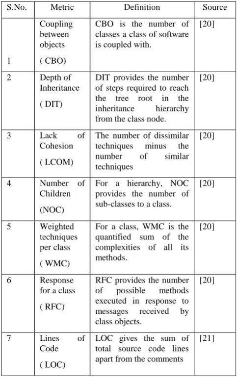
Table 1: Metrics used in the study
S.No. Metric Definition Source
1
Coupling between objects
( CBO)
CBO is the number of classes a class of software is coupled with.
[20]
2 Depth of Inheritance
( DIT)
DIT provides the number of steps required to reach the tree root in the inheritance hierarchy from the class node.
[20]
3 Lack of
Cohesion
( LCOM)
The number of dissimilar techniques minus the number of similar techniques
[20]
4 Number of Children
(NOC)
For a hierarchy, NOC provides the number of sub-classes to a class.
[20]
5 Weighted techniques per class
( WMC)
For a class, WMC is the quantified sum of the complexities of all its methods.
[20]
6 Response for a class
( RFC)
RFC provides the number of possible methods executed in response to messages received by class objects.
[20]
7 Lines of
Code
( LOC)
LOC gives the sum of total source code lines apart from the comments
This study uses OO metrics provided by Chidamber & Kemerer as they are the most widely used metrics in the literature [20-22].
Table 1 lists the metrics utilized in this paper [20]. The values of these metrics have been extracted using Understand for Java software. (http://www.scitools.com/)
3.2
Dependent Variable
The dependent variable is the behavior of the software which is being observed by the researchers. In this study, change proneness of the software is the dependent variable. As defined in [17], change proneness is the likelihood of change in a class in the subsequent releases of the software. It can be quantified by analyzing the lines of code that have been added, deleted or modified. The detailed technique for determination of change proneness of a class has been described in section 4.
4.
EMPIRICAL DATA COLLECTION
In this section, the procedure used for data collection for all the software projects under analysis has been stated.
4.1
Data Collection Procedure
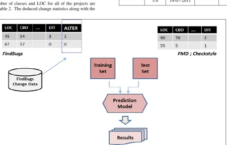
Three open source software have been used as the software projects under analysis. The projects are – FindBugs, PMD and checkstyle and the source code is available on www.sourceforge.net. These projects have been developed in Java language and belong to a similar application domain i.e. source code analyzers. The change data from two versions of each of the software projects is taken to empirically validate the process of change proneness prediction. The change data accounts for the various defect removals and enhancements that a project undergoes in the subsequent versions of software. The details of each software such as version, release date, number of classes and LOC for all of the projects are listed in table 2. The deduced change statistics along with the
OO metrics constitute the data points for the development of the prediction models.
A number of steps are followed to collect data from the software projects under analysis. A more detailed method of data collection can be referred from Malhotra et al. [17]. The first step is to compute the independent variables of the three projects. The independent variables i.e. OO metrics, are collected from the previously released version of each of the projects using the Understand for Java software. The metrics of unknown classes, methods, files are ignored and the information about of the required classes is extracted. The second step is the generation of the comparable versions of each of the software projects. These versions are generated by processing the two releases of the software projects under analysis and extracting the classes common to both the versions. A variable named ‘ALTER’ which holds binary values- ‘1’ if there are one more changes in a common class of the software project, ‘0’ is there is no difference in that class of both the releases. The methodology followed to process these versions and evaluate the variable ALTER is in accordance with that of Malhotra et al. [17].
Table 2 Software Details
Name Version Release date LOC Classes
FindBugs 1.2.1 31-5-2007 82827 849 1.3.9 21-08-2009 1,10,907 1080
PMD
3.9 19-12-2006 71,114 822
4.0 20-07-2007 54,031 679
Checkstyle
5.3 19-10-2010 52,360 792
[image:3.595.88.540.447.736.2]5.4 14-07-2011 52,888 796
For FindBugs, there were 555 common classes between the two releases. Thus, the change data of these classes combined with their OO characteristics yield 555 data points. Similarly, analysis of PMD and Checkstyle generated 432 and 212 data points respectively as shown in Table 3.
For the empirical validation of inter project change prediction, FindBugs has been used as the input training set, as it provides a large number of data points for training. The models built using this data set have then been separately tested on the data points provided by the other software projects under analysis- PMD and Checkstyle. The method used for inter project validation in this study has been depicted in Figure 1.
Table 3: Details of generated data points
Name of the software No. of data points generated
FindBugs 555
PMD 432
Checkstyle 212
5.
RESEARCH METHODOLOGY
The following section states the techniques used for analysis of the data points acquired using the data collection procedure.
5.1
Correlation based feature selection
In order to develop effective prediction models, one requires a representative input set of variables that can be used. Such an input set is achieved through Correlation Based Feature Selection (CFS), which removes the unwanted or noisy features from the inputs. This results in decrease of dimensionality of the feature set yielding an optimal number of inputs. It can reduce the time of execution and improve the efficiency of such models [23]. This paper explores the effectiveness of three types of techniques for inter project change proneness prediction, namely statistical, machine learning (ML) and AIS techniques. Section 5.1.1 describes the statistical technique used, Sections 5.1.2- 5.1.4 describe the machine learning techniques and Sections 5.1.5- 5.1.7 describes the AIS techniques used in the study. The default settings provided in the WEKA tool for the ML and that of the WEKA plugin for AIS techniques have been used [28].
5.1.1
Logistic Regression
Logistic Regression (LOG) is a statistical technique useful in modeling the relationship between a dependent variable and a set of independent variables. It differs from linear regression as the logistic function determines probabilities of the occurrence of an event as opposed to the prediction of change in dependent variable. [24] The probabilities are modeled as a function of the specified inputs. The formula for logistic regression is as follows:
5.1.2
Bagging
In Bootstrap aggregating (BAGG) technique, replicates of the training set are produced through sampling. For the learning data of size m, the method creates bootstrap samples of size less than m. The individual results of all the models are then assembled and the records are stored. The accuracy of this technique is dependent on the significance of the selected training data [25]. The default settings used in WEKA tool
are 10 iterations, bag size percent of 100 and REP tree as the classifier.
5.1.3
Adaptive Boosting
Adaptive Boosting (ADA) is a popular ensemble algorithm which is commonly used for boosting methods. It is applied to learn weak classifiers and derive a stronger performance classifier from the individual classifiers [26]. On the basis of performance, weights are assigned to the individual weak learners and expertise is gained by analyzing the incorrect classifications made by the previous models. The accuracy of this algorithm wavers with noisy data. The WEKA default settings were applied with 10 iterations and weight mass percentage of 100 used to build the classifiers.
5.1.4
Bayesian Network
In Bayes Net (BN) algorithm, a network is created which comprises of a set of individual nodes and directed edges connection them [27].This network aids in the determination of the relationship between random variables and probabilistic values of the relationship dependency. The technique is useful when there is uncertainty in the problem domain, regarding the relationship between the input variables. It investigates the strength of the connections between the variables quantitatively. The final result is the joint probabilistic distribution derived from the network. A simple estimator and K2 search algorithm have been used as the default settings in WEKA tool.
5.1.5
AIRS1
Inspired from biological computation and artificial intelligence, it is a supervised learning algorithm. The first involves initialization followed by artificial recognition ball (ARB) generation, competing for resources and memory cell identification. The detail of the methodology can be seen in [28]. The default settings of the plug in of WEKA for AIRS have been used. The algorithm is operated at an affinity threshold scalar of 0.2 and clonal rate of 10.0.
5.1.6
AIRS2Parallel
AIRS2Parallel (A2P) operates in parallel through partitioning and can be used to get a speedup in the levels of classification accuracy [29]. This technique differs from AIRS1 in relation to the mannerism in which clones are mutated and value of different user parameters like simulation value. A merging scheme is used to jointly classify from the various individual memory pools of the partitions. The settings in WEKA include a clonal rate of 10.0 and hyper mutation rate of 2.0.
5.1.7
Clonal Selection Classifier Algorithm
Clonal selection classifier algorithm (CSCA) is a classification algorithm developed by Brownlee [30], inspired by the CLONALG algorithm and its variants. It can be expressed as a fitness function where the goal is to maximize the accuracy of classification and minimize that of misclassification. The settings used in WEKA are a clonal scale factor of 1.0 and initial population size of 50.6.
ANALYSIS & RESULTS
This section concludes the observations made by the performance of the prediction models on the given data sets using logistic, machine learning and AIS techniques. The effectiveness of the prediction models have been evaluated by the following parameters [17]:
change. High value of sensitivity indicates a good prediction technique for change proneness.
2. Specificity: It is the percentage of ratio of classes that were incorrectly predicted to exhibit change. Values of sensitivity and specificity in closest proximity to each other yield the cutoff point which is the optimal points in analysis of the models.
3. Receiver Operating Characteristic (ROC) Analysis: ROC curve is utilized as a measure for prediction in ROC analysis with 1- specificity as the x coordinate and sensitivity as the y coordinate [18]. The area-under-curve (AUC) helps in determining the prediction accuracy of the model.
4. Ten-cross validation: In n cross validation, the input data set is divided into n sub data sets where n-1 sets are operated upon as training sets to analyze the nth set which is the test set. To make the statistical tests results more reliable, a ten cross validation was performed on all the data sets. [31]
In the following subsections, results of the analysis are stated.
6.1
Descriptive Statistics
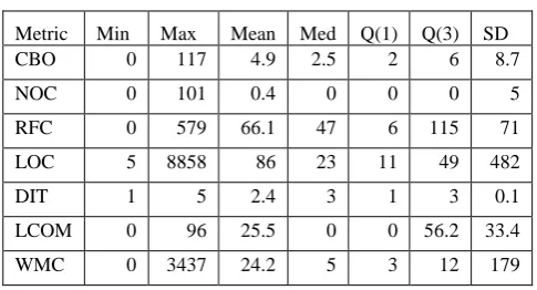
Tables 4, 5 and 6 provide the detailed statistics of the considered metrics in this study. These include the minimum (Min), maximum (Max), Mean, Median (Med), 1st Quartile (Q1), 3rd Quartile (Q3) and standard deviation (SD). Some of the data characteristics are as follows:
1. Size of the three software projects is diverse with a range of 5 to 2724 LOC for Checkstyle with mean of 104 LOC, PMD has range from 5 to 8858 LOC and mean of 87 LOC. The software which is used as the training set for both the mentioned projects, FindBugs, has a range from 7-553 LOC with a mean of 83 LOC.
2. LCOM holds high values of upto 100 in all the sets.
3. Low levels of inheritance can be observed in all projects with low mean values of NOC (0.1 for Findbugs, 0.4 for PMD and 0.3 for Checkstyle.) and DIT ( 3.5 for Findbugs, 2.4 for PMD and 2.3 for Checkstyle.). The results are similar to studies in related fields [11-13].
[image:5.595.306.549.95.226.2]Table 4: Metric Statistics for FindBugs
[image:5.595.304.549.260.391.2]Table 5: Metric Statistics for PMD
Table 6: Metric Statistics for Checkstyle
6.2
Inter project validation results for
PMD
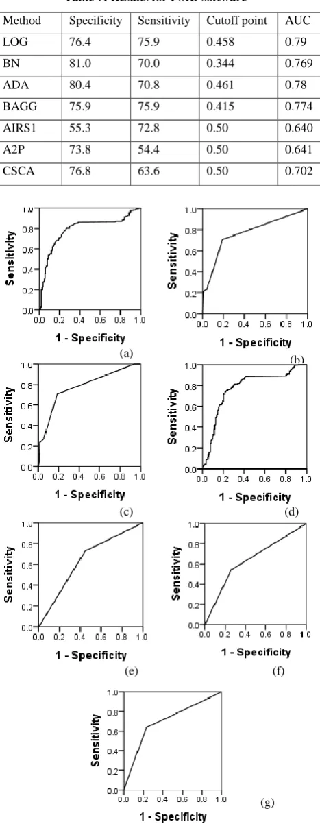
In order to evaluate inter project validation, the authors use FindBugs as the training set and PMD as the test set. For using PMD as the test set, data points from the FindBugs dataset formed the training set. CFS was applied to the input set to get the optimal combination of metrics. The metrics selected after applying CFS technique were CBO, LOC and WMC. The data points of the PMD software were added as inputs to the model generated using the FindBugs software using the WEKA tool and the performance of different techniques has been observed as in table 7.
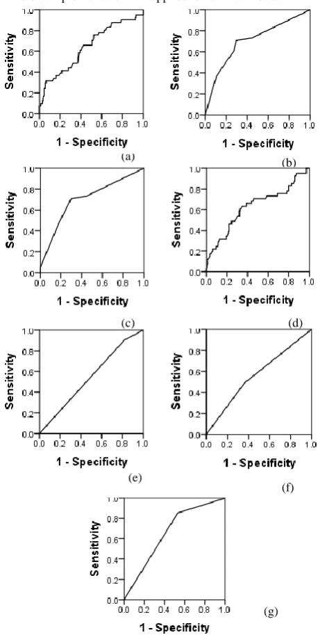
The model developed using LOG gave good results with an AUC measure of 0.79 and high values of specificity and sensitivity of 76.4% and 75.9% respectively. The cut-off point recorded by LR was at 0.458. The models generated using the BN and ADA techniques showed similar outputs with an AUC measure of 0.769 and 0.78 respectively and cut off points of 0.344 and 0.461 respectively. Both techniques displayed high values of specificity of 81% and 80.4% respectively. The cutoff point of BAGG model was 0.415 with both specificity and sensitivity values being 75.9%. The BAGG model displayed a comparable AUC measure of 0.774. The results provided by models developed using the Artificial Immune System (AIS) techniques were discouraging with an AUC measure of 0.64 shown by AIRS1 technique. Model using the AIRS1 technique displayed dissimilar values of sensitivity and specificity of 72.8% and 55.3% respectively at a cut-off point of 0.5. The A2P technique showcased contrasting values with good specificity value of 73.8% but low sensitivity value of 54.4%. The model developed using CSCA provided relatively good results with an AUC measure of 0.704 and specificity and Metric Min Max Mean Med Q(1) Q(3) SD
CBO 0 117 4.9 2.5 2 6 8.7
NOC 0 101 0.4 0 0 0 5
RFC 0 579 66.1 47 6 115 71
LOC 5 8858 86 23 11 49 482
DIT 1 5 2.4 3 1 3 0.1
LCOM 0 96 25.5 0 0 56.2 33.4
WMC 0 3437 24.2 5 3 12 179
Metric Min Max Mean Med Q(1) Q(3) SD
CBO 0 27 3.3 3 2 4 3.1
NOC 0 16 0.1 0 0 0 1.3
RFC 1 88 37.9 43 30 51 18.1
LOC 7 553 83 56 32.75 112 76.7
DIT 1 7 3.5 4 2 4 1.5
LCOM 0 100 42.4 50 0 77 36.7
WMC 1 106 14.4 10 5 19 13.6
Metric Min Max Mean Med Q(1) Q(3) SD
CBO 0 62 6.3 4 2 7 8.1
NOC 0 79 0.3 0 0 0 3.4
RFC 1 309 43 12 5 40.5 62.7
LOC 5 2724 104 52 24 110 185
DIT 1 7 2.3 1 1 3 1.8
LCOM 0 100 49.3 55 22.5 78 33
(b) (a)
(c) (d)
(e)
[image:6.595.52.286.126.728.2]sensitivity of 76.8% and 63.6% respectively. The statistical and machine learning techniques indicate comparable performance. Their performance can be analyzed through ROC curves in Figure 2.
Table 7: Results for PMD software
Method Specificity Sensitivity Cutoff point AUC
LOG 76.4 75.9 0.458 0.79
BN 81.0 70.0 0.344 0.769
ADA 80.4 70.8 0.461 0.78
BAGG 75.9 75.9 0.415 0.774
AIRS1 55.3 72.8 0.50 0.640
A2P 73.8 54.4 0.50 0.641
CSCA 76.8 63.6 0.50 0.702
Fig. 2: ROC curves for PMD Software Models: a.LOG b. BN c. ADA d. BAGG e. AIRS1 f. A2P g. CSCA
6.3
Inter Project Results for Checkstyle
After applying the CFS technique to the training set provided by the FindBugs data set, the metrics extracted to form the feature set were CBO, LOC and WMC. The metrics data from the Checkstyle software gives the inputs required for the test set. The results displayed by the models developed using the different techniques have been shown in table 8.
The best results were shown by the model using the BN technique with an AUC measure of 0.704 and good values of sensitivity and specificity of 70.7% and 70.2% respectively. The cut-off point for the BN technique was at 0.510. The ADA technique displayed similar results with a higher cut-off point of 0.604. The model developed using the LR technique exhibited low results with an AUC measure of 0.642. The specificity and sensitivity of the LR model was 60.8% and 61.0% respectively. The model using BAGG technique displayed comparable results with low sensitivity and specificity of 63.4% and 63.2% respectively at a cut-off point of 0.591 and AUC measure of 0.629. The AIS models exhibited disappointing results with the best results showcased by the model developed using the CSCA technique with an AUC measure of 0.661. The CSCA model showed high sensitivity of 85.4% but very low specificity of 46.8% at a cut-off point of 0.5. The model using the AIRS1 and A2P techniques exhibited extremely low AUC measures of 0.542 and 0.563 respectively. The A2P model showed specificity and sensitivity of 63.7% and 51.2% respectively. The ROC curves of all the models developed for Checkstyle as the test set can be seen in Figure 3.
Table 8: Results for Checkstyle software
7.
THREATS TO VALIDITY
This section is used to describe the possible threats to the validity of the work.
7.1
Construct Validity
Construct validity depends on the usage of the dependent & independent variables and the methods used to determine them. The dependent variable in this study is a binary variable which has been calculated manually and thus does not provide any threats. However, this study does not categorize whether the change occurred was corrective, adaptive, perfective or preventive in nature as in [32]. This could be a possible source of threat.
7.2
External Validity
In this study, three open source software have been analyzed from similar application domain to decrease the threat of external validity. However, it still poses a threat as generalization cannot be concluded unless the same Method Specificity Sensitivity Cutoff point AUC
LOG 60.8 61.0 0.467 0.642
BN 70.2 70.7 0.510 0.704
ADA 70.2 70.7 0.604 0.703
BAGG 63.2 63.4 0.591 0.629
AIRS1 18.1 90.2 0.500 0.542
A2P 63.7 51.2 0.500 0.563
CSCA 46.8 85.4 0.500 0.661
(f)
(a)
(b)
(c) (d)
(e)
procedure is replicated across a number of data sets with different implementation and application environments.
Fig. 3: ROC curves for Checkstyle Software Models: a. LOG b. BN c. ADA d. BAGG e. AIRS1 f. A2P g. CSCA
8.
CONCLUSION AND FUTURE WORK
The study aimed at the investigation of the applicability of inter project validation to detect change prone classes in a software. The work was validated using three software projects in which the Findbugs software data set was used as the training set and PMD and Checkstyle software data sets were used as the test sets. The models developed to predict change proneness were developed using a range of popular logistic and machine learning techniques and some unexplored AIS techniques.
The effect of OO metrics on change proneness in software was also analyzed and their relation comprehended. The conclusion of the study are stated as follows:
1. The results exhibited by the prediction models demonstrate that in the absence of prior historical data, software can be tested for change proneness
on models built using statistics from other project data. This is known as inter project validation. Such techniques can help developers to predict the change prone modules of a software in the absence of complete project data. This can be utilized to make the software testing process more efficient in terms of both time and resources.
2. The accuracy of logistic and machine learning techniques for predicting change proneness in inter- projects is comparable with BN and LR showing good results with high values of specificity and sensitivity. The AIS algorithms which exploit the characteristics displayed by the immune systems prove ineffective in their classification accuracy for inter-project validation.
3. The CBO, LOC and WMC metrics indicate strong correlation with the dependent variable of the study, i.e. change proneness. This can be seen by their selection in the input feature set using the CFS method.
These observations are valid for medium- sized object oriented systems. The authors plan to further generalize the applicability of inter project validation across diverse language and application environments and discover the most effective techniques for analyzing such models.
9.
REFERENCES
[1]S. Watanbe, H. Kaiya and K. Kaijiri, “Adapting a Fault Prediction Model to Allow Inter Language Reuse,” PROMISE Proceedings of the 4th international workshop on Predictor models in software engineering 2008, (2008) pp. 19-24.
[2]W. Li and S. Henry, “Object Oriented Metrics that Predict Maintainability”, Journal of Systems and Software, vol. 23 ,(1993) pp. 111-122.
[3]L. Briand, J. Wust and H. Lounis,“Replicated Case Studies for Investigating Quality Factors in Object Oriented Designs.” Empirical Software Engineering: An International Journal, vol. 6 ,(2001) pp. 11-58.
[4]V.R. Basili, L.C. Briand and W.L. Melo, “A Validation of Object- Oriented Design Metrics as Quality Indicators,” IEEE Transactions on Software Engineering, vol. 22, no. 10 , (1996) pp. 751-761.
[5]Y. Singh, A. Kaur and R. Malhotra. “Empirical Validation of Object-Oriented Metrics for Predicting Fault Proneness,” Software Quality Journal, vol. 18, no.1, (2010) pp. 3-35.
[6] R. Kohavi and D. Sommerfield, “Targeting Business Users with Decision Table Classifiers,” Proceedings of IEEE Symposium on Information Visualization, (1998) pp. 102-105.
[7]K. Michalak and H. Kwasnicka,“Correlation-based Feature Selec-tion Strategy in Neural Classification,” Sixth International Conference on Intelligent Systems Design and Applications, vol. 1, (2006) pp. 741-746.
[8]B. Kitchenham, L. Mendes, “A Systematic Review of Cross- vs. Within-Company Cost Estimation Studies”, IEEE Transactions on Software Engineering, vol. 33, no. 5, (2007) pp. 316-329.
(f)
[image:7.595.52.283.91.548.2][9]T. Zimmermann, N. Nagappan, H. Gall, E. Giger and B. Murphy, “Cross-project Defect Prediction A Large Scale Experiment on Data vs. Domain vs. Process”, in Proceedings of the 7th joint meeting of the European Software Engineering Conference and the ACM, (2009) pp. 91–100.
[10] G. Canfora, A.D. Lucia, “Multi-objective cross project defect prediction”, Software Testing, Verification and Validation (ICST), 2013 IEEE Sixth International Conference, (2013) pp. 252-261.
[11] Z.He, F.Shu, An investigation on the feasibility of cross-project defect prediction”, Automated Software Engineering, vol. 19, no.2, (2012) pp. 167-199.
[12] A.R. Han, S. Jeon, D. Bae and J. Hong,“ Behavioral Dependency Measurement for Change Proneness prediction in UML 2.0 Design Models,” Computer Software and Applications 32nd Annual IEEE International, (2008) pp.76-83.
[13] O. Elish, Al Rahman, “A suite of metrics for quantifying historical changes to predict future change-prone classes in object-oriented software.” Journal of Software: Evolution And Process. J. Softw.: Evol. and Proc., vol.25, (2013) pp. 407–437.
[14] Zhou Y, Leung H, Xu B “Examining the potentially confounding effect of class size on the associations between object oriented metrics and change proneness”, Software Engineering, IEEE Transactions, vol. 35 , no. 5 , (2009), pp. 607-623.
[15] H. Lu, Y. Zhou, B. Xu, H. Leung and L. Chen, “The ability of object-oriented metrics to predict change-proneness: a meta-analysis”, Empirical Software Engineering Journal June 2012, vol. 17, no. 3, (2012) pp. 200-242.
[16] M. D'Ambros, M. Lanza and R. Robbes, “On the Relationship Be-tween Change Coupling and Software Defects,” 16th Working Conference on Reverse Engineering, (2009) pp. 135-144.
[17] R. Malhotra and M. Khanna, “Investigation of Relationship be-tween Object-oriented Metrics and Change Proneness,” International Journal of Machine Learning and Cybernetics, Springer vol. 4, no. 4, (2013) pp. 273-286.
[18] R. Malhotra and M. Khanna, “Inter Project Validation for Change Proneness Prediction using Object Oriented Metrics,” Software Engineering- An International Journal , vol. 3, no. 3 (2012) pp. 21-31.
[19] Kerlinger, F. N. Foundations of behavioral research (3rd ed.). Fort Worth: Holt, Rinehart and Winston, Inc.(1986)
[20] S. R. Chidamber and C.F. Kemerer,“A Metrics Suite for Object Ori-ented Design,” IEEE Transactions of Software Engineering, vol. 20, no.6 (1994)pp. 476-493.
[21] KK. Aggarwal, Y. Singh, A. Kaur and R. Malhotra, “Empirical Analysis for Investigating the Effect of Object-Oriented Metrics on Fault Proneness: A Replicated Case Study”, Software Process: Improvement and Practice, vol. 16, no. 1, (2009) pp. 39-62.
[22] Basili VR, Briand LC, Melo WL “A validation of object oriented design metrics as quality indicators”, IEEE Trans Softw. Engg , vol. 22, no. 10, (1996) pp. 751–761.
[23] Hall MA, “Correlation-based feature selection for discrete and numeric class machine learning”, proceeding of the seventeenth international conference on machine learning, (2010) pp. 359–366.
[24] Hosmer D, Lemeshow S -Applied logistic regression. Wiley, New York, (1989).
[25] Kristína Machová, František Barčák, Peter Bednár- A Bagging Technique using Decision Trees in the Role of Base Classifiers, (2006).
[26] Yoav Freund Robert E. Schapire. -A short introduction to boosting, (2009).
[27] Ben-Gal I., Bayesian Networks, in Ruggeri F., Faltin F. & Kenett R., Encyclopedia of Statistics in Quality & Reliability, Wiley & Sons, (2007).
[28] C. Catal, B.Diri,”An Artificial Immune System Approach for Fault Prediction in Object-Oriented Software”, Dependability of Computer Systems, 2007. DepCoS-RELCOMEX '07. 2nd International Conference, (2007) pp. 238-245.
[29] Brownlee, J.- Artificial Immune Recognition System (AIRS) A review & Analysis, Technical Report 1-02, Swinburne University of Technology, Australia, (2005).
[30] Khalid A, H.M. Abdul, “Artificial Immune Clonal Selection Classification Algorithms for Classifying Malware and Benign Processes Using API Call Sequences”, IJCSNS, (2010) pp. 31-39.
[31]L. Briand, J. Wust, J. Daly and D.V. Porter, “ Exploring the Relationships between Design Measures and Software Quality in Object-oriented Systems,” Journal of Systems and Software, vol. 51, no.3, (2000) pp. 245-273.