Path dependent volatility

Munich Personal RePEc Archive

Path dependent volatility

Pascucci, Andrea and Foschi, Paolo

Università di Bologna

30 November 2006

Online at

https://mpra.ub.uni-muenchen.de/973/

Path dependent volatility

Paolo Foschi and Andrea Pascucci

Dipartimento di Matematica, Universit`a di Bologna ∗

Abstract

We propose a general class of non-constant volatility models with dependence on the past. The framework includes path-dependent volatility models such as that by Hobson&Rogers and also path dependent contracts such as options of Asian style. A key feature of the model is that market completeness is preserved. Some empirical analysis, based on the comparison with the performance of standard local volatility and Heston models, shows the effectiveness of the path dependent volatility.

1

Introduction

In the Black-Merton-Scholes option pricing theory [3], [19], the underlying asset is modeled as a geometric Brownian motion whose dynamic under the risk neutral measure is given by

dSt=rStdt+σStdWt. (1.1)

In (1.1)rdenotes the locally riskless interest rate andσis the volatility. Under the assumption that

both the parameters are constant, model (1.1) leads to closed formulas for plain vanilla options. Nowadays the Black&Scholes formula is widely used in practice, to the extent that prices of call and put options are usually quoted in terms of the so-called Black&Scholes implied volatility. However it is also apparent that the prices at which derivatives are traded are inconsistent with the assumption of a constant volatility: indeed especially after the market crash of 1987, the strong empirical evidences of the stochastic nature of the volatility stimulated the development of more realistic models. The overall aim of a non-constant volatility model is twofold: on one hand, to produce prices of plain vanilla options which agree with the observed volatility surfaces and to price exotic options consistently; on the other hand, to find the correct replicating strategy in order to improve the hedging performance.

The first task is usually not difficult to achieve: from a theoretical point of view, any model which depends on a sufficiently large number of parameters can be calibrated to fit (or at least approximate) market prices. But it should be emphasized that any calibration procedure depends on the quantity and quality of the available data: in particular, since only option prices correspond-ing to a finite number of maturities and strikes are quoted, generally the fittcorrespond-ing of prices cannot usually be done in a unique way. Then the essential and hard problem is to determine the “correct” hedging strategy: indeed it is well-known that the hedge parameters are strongly model-dependent even for call and put options (cf. for instance [7]).

From this point of view, the widely used local volatility (henceforth LV) models give poor results. In a LV model the volatility is supposed to be a deterministic function of the time and current price of the underlying asset. The main advantages are that the market is complete and in principle it is possible to specify the volatility function in such a way that option prices given by

the model agree with market prices. On the other hand the empirical study by Dumas, Fleming and Whaley [10] shows that, for hedging purposes, the local volatility underperforms an ad-hoc use of the Black&Scholes model (which consequently should be preferable for its parsimony). The conclusion in [10] is that, as far as one aims to preserve market completeness, a volatility model depending on the whole past trajectory of the asset (instead of the current price alone) should be investigated.

The first results in this direction were obtained by Hobson and Rogers who proposed in [16] a volatility model defined in terms of the difference between the current price and an exponentially weighted average of past prices. Section 2 is devoted to a brief review of this model. We also discuss the main positive aspects and the possible weak points of the Hobson&Rogers model.

The aim of this paper is to propose a general notion of path dependent volatility which in

our opinion overcomes some of the mathematical and economical problems of the Hobson&Rogers model. This is done in Section 3 where we also prove some results about the absence of arbitrage and completeness of the market in the framework of PDEs and martingales theories. Then in Section 4 we analyze some suitable transformation of the pricing PDE which seems to be more convenient for the numerical approximation.

In Section 5 the path dependent volatility model is validated against market data and the per-formance compared with those of standard LV and Heston stochastic volatility models. Specifically our aim is to compare the performance of the hedging strategies produced by the models in different market scenarios. To this end we examine the market reversal in May 2006 and observe that a path dependent volatility generally outperforms LV and Heston models: in particular it turns out that the tracking errors of Heston minimum-variance hedging are up to twice the hedging errors of a path dependent volatility model, especially after sudden market movements.

2

The Hobson&Rogers model

In this section we recall the main features of a simplified version of the Hobson and Rogers model

[16]. In a Wiener space with one-dimensional Brownian motionW, we denote byStthe stock price

and by Mt and Dtrespectively the trend and thedeviation processes defined by

Mt=λe−λt

Z t

−∞

eλsZsds, λ >0 (2.1a)

and

Dt=Zt−Mt, (2.1b)

where Zt = log(e−rtSt) is the log-discounted price process. The function eλs in (2.1) is called the

average weight: the parameterλdescribes the rate at which past prices are discounted.

Hobson and Rogers assume that St is an Itˆo process, solution to the stochastic differential

equation (SDE)

dSt=µ(Dt)Stdt+σ(Dt)StdWt. (2.2)

In (2.2), µand σ >0 are deterministic functions satisfying usual hypotheses in order to guarantee

that the system of SDEs (2.1)-(2.2) has a solution. A key feature of the model is that the process

(St, Dt) is Markovian (cf. Lemma 3.1 in [16]). Thus, the price of an option, with maturity T, can

be obtained in terms of solution to the following Cauchy problem (cf. [13]):

σ2(x₋y)

2λ (∂xxu−∂xu) + (x−y)∂yu−∂tu= 0, inR

2

×[0, λT], (2.3)

Path dependent volatility models are supported by the empirical evidence about the dependence

of the volatility with respect to the deviationD: Figure 1 plots implied volatilities against adjusted

log-moneyness for options on the S&P 500 index in the years 2003-2004. The implied volatilities are

grouped by ranges of values of D. It is immediate to observe on the figure that implied volatilities

increase as theDdecreases (see also the empirical analysis in [20], Section 2). This enlightens the

well-known negative correlation between volatility and market prices.

−0.25 −0.2 −0.15 −0.1 −0.05

Dev. from trend

−0.5 0 0.5 0.15 0.2 0.25 0.3 0.35 0.4 0.45 0.5 Moneyness Implied Volatility

−0.25 −0.2 −0.15 −0.1 −0.05

Dev. from trend

−0.5 0 0.5 Moneyness

−0.25 −0.2 −0.15 −0.1 −0.05

Dev. from trend

−0.5 0 0.5 Moneyness

−0.25 −0.2 −0.15 −0.1 −0.05

Dev. from trend

−0.5 0 0.5 0.15 0.2 0.25 0.3 0.35 0.4 0.45 0.5 Moneyness

Figure 1: Effects of the deviation from the trend on marked implied volatilities. The implied volatilities are

plotted against adjusted log-moneyness log(F/K)/√T−tand grouped by different ranges of Dtas shown

by the bar in the top of each panel. Data from the S&P 500 index options, years 2003-2004.

We emphasize that no additional source of risk has been added in the Hobson&Rogers model: therefore, unlike many other non-constant volatility models, the market is complete and the arbi-trage argument which underlies the Black&Scholes theory is preserved. While keeping the market completeness, the Hobson&Rogers model is able to approximate observed volatility surfaces (see the analysis in [13]).

We also remark that a path dependent volatility incorporates information on the past and then, once it is calibrated to the market, the model somehow “knows” the behaviour of investors in different market circumstances and can also keep into account of the positive or negative trend of the asset. For instance, unlike standard local or stochastic volatility models, in case of a sudden fall of the market a path dependent volatility model is designed to automatically increase the level of volatility in order to undertake the market dynamics in a more natural way. This is the reason why it seems that path dependent volatility models do not need to be continuously re-calibrated (which is a well-known disadvantage of local volatility models) and have better out-of-sample performances (see analysis in [13]).

Thanks to these fine features, the Hobson&Rogers model raised some interest mainly among

academics: the problem of parameters calibration (λ in the average weight and the volatility

function σ) was studied by Platania and Rogers [20], Fig`a-Talamanca and Guerra [12] and us

in [13]. Di Francesco and one of the authors studied the numerics of the model: we explicitly

remark that the PDE in (2.3) is not uniformly parabolic even if it is hypoelliptic by H¨ormander’s

theorem [17]. In particular the convergence of finite difference schemes does not follow by standard arguments but it is proved in [8] as a consequence of some a priori estimates for solutions to (2.3)-(2.4) provided in [9].

smiles. The robustness of the Hobson&Rogers model with respect to the data and parameters was studied by Hallulli and Vargiolu [4].

Next we mention some of the weak points of the Hobson&Rogers model. As noted in [4], some

mathematical and economical concerns arise from the definition of the deviation processDin (2.1).

Indeed D involves the path of the underlying asset on all its past ]_{− ∞}, t[. The requirement of

an infinite horizon in the past obviously raises practical problems since only finite time series are available so that misspecifications in the model are unavoidable. To overcome this problem, in [4] the following extension of the Hobson&Rogers model has been proposed: the volatility is specified as

σ(St) =σ(St, Yt, St−τ)

where

Yt=

Z t

t−τ

e−λ(t−v)_f(S

v)dv,

where f is a strictly monotone function and τ is a given delay parameter. Unfortunately the

conclusion in [4] is that ifτ is finite then the previous model cannot admit a Markovian realization

so that it loses any appeal.

As a further remark, it seems that the average weight λe−_λt

in (2.1) is not flexible enough to take into account of the special properties of the underlying process that may arise, for instance, from stagionality effects, fusions of stocks, capitalization changes.

In this paper we focus on these problems: we propose a simple generalization of the Hob-son&Rogers model and introduce a new class of models for asset prices with volatility dependent

on the past. Our idea is to consider a more flexible deviation process defined in terms of ageneric

average weight, possibly corresponding to a finite time horizon. We call this the path dependent

volatility (henceforth PDV) model. The notion of PDV model is sufficiently general to include the Hobson&Rogers model and also path dependent derivatives such as Asian style options.

We conclude this section with a further remark. In a PDV model the market is complete since no new sources of randomness are introduced: then we have the apparent advantage that there are unique preference-independent prices for contingent claims. The drawback is that market completeness is barely considered a realistic assumption. In a PDV model options are in principle redundant in that they can be perfectly replicated by delta-hedging in the underlying asset. Then in this framework trading strategies that hedge against volatility risk (for instance, vega-hedging using traded options) are meaningless from a theoretical point of view. An obvious idea is to investigate jump-diffusion or truly stochastic volatility models in the framework of PDV and we aim to come back to this point in a forthcoming paper.

3

Path dependent volatility

In order to introduce the PDV model, we consider an average weight ϕ which is a non-negative,

piecewise continuous and integrable function on ]_−∞, T]. We also assume thatϕis strictly positive

in [0, T] and we set

Φ(t) =

Z t

−∞

ϕ(s)ds.

Then we define the average process as

Mt=

1 Φ(t)

Z t

−∞

where Zt = log(e−rtSt) denotes the log-discounted price process. Typical specifications of the

average weights are given by following examples:

- ϕ(t) =eP(t)_{max{Q(t),0}where P, Qare suitable polynomial functions: the Hobson&Rogers}

model corresponds toP(t) =λtand Q(t) = 1;

- ϕ(t) = 1 for t _∈ [0, T] and null elsewhere: this corresponds to the geometric average of an

Asian option;

- ϕpiecewise linear function.

We remark that

dMt=

ϕ(t)

Φ(t)(Zt−Mt)dt; (3.1)

then by assuming the following dynamic for the asset log-price

dZt=µ(Zt−Mt)dt+σ(Zt−Mt)dWt, (3.2)

we deduce that, under standard hypotheses on the coefficientsµ, σ,the couples (Z, M) and (Z, D)

are Markovian processes. Actually in the sequel we restrict ourselves to a Markovian setting and we denote by

Vt=α(t, Zt, Mt)St+β(t, Zt, Mt)Bt (3.3)

the value of a portfolio, where α, β are suitably regular (deterministic) functions and Bt = ert.

Moreover we set

f(t, Zt, Mt) =B

−₁

t Vt (3.4)

the discounted value ofV. The next theorem characterizes the self-financing strategies.

Theorem 3.1. The following conditions are equivalent:

1. the portfolio in (3.3) is self-financing;

2. the function f in (3.4) solves the partial differential equation

σ2_(z−m)

2 (∂zzf −∂zf) +

ϕ(t)

Φ(t)(z−m)∂mf +∂tf = 0 (3.5)

in ]0, T[_×R2, and the following relations hold

α(t, z, m) =e−z_∂

zf(t, z, m), β(t, z, m) =f(t, z, m)−e−z∂zf(t, z, m). (3.6)

Proof. By the self-financing condition, it holds

df =₋rf dt+B−₁

t (αdSt+βdBt) =

(sinceβdBt=rβBtdt=r(Vt−αSt)dt)

=αB−₁

(since, by Itˆo formula,dSt=BteZt

dZt+

r+ σ₂2dt)

=αeZt

dZt+

σ2

2 dt

. (3.7)

On the other hand, by Itˆo formula and (3.1), we get

df(t, Zt, Mt) =

∂tf +

σ2

2 ∂zzf+

ϕ

Φ(Zt−Mt)∂mf

+∂zf dZt. (3.8)

Comparing (3.7) and (3.8), by the uniqueness of the representation of an Itˆo process, we infer

∂zf(t, Zt, Mt) =α(t, Zt, Mt)eZt. (3.9)

Now we recall that, since by assumptionϕis strictly positive on [0, T], the conditions of the classical

H¨ormander’s theorem are satisfied and the process (Zt, Mt) has astrictly positivedensity onR2 for

t > 0 (we also refer to the paper [9] by Di Francesco and one of the authors for a direct proof of

this result). Then (3.6) readily follows from (3.9). Analogously, by equating the dt-parts of (3.7)

and (3.8) and using (3.9), we obtain the PDE (3.5).

We do not prove the inverse implication which is straightforward.

Next we prove that in the PDV model the market is arbitrage-free and complete.

Corollary 3.2. For any contingent claim H =H(ST, MT), with H ∈L1_loc(R2) and H ≥0, there exists a unique self-financing and admissible1 strategy replicatingH. The strategy is determined by formulas (3.6) where f is the unique solution of the Cauchy problem for equation (3.5) with final condition

f(T, z, m) =e−rT_H(ez_{, m). (3.10)}

In particular, the market is arbitrage-free and complete: Ht:=ertf(t, Zt, Mt) is the arbitrage price of the claim H.

Proof. The thesis is a direct consequence of Theorem 3.1 and of the existence and uniqueness results for degenerate parabolic equations of Kolmogorov type (which include (3.5)) proved by Di Francesco and one of the authors [9] and by Polidoro [21].

The previous results can be also proved by using the martingale theory. Note that the dynamic

of the stock priceSt is given by

dSt=

r+µ(Dt) +

σ2_(D

t)

2 St

dt+σ(Dt)StdWt

where the deviation process Dt=Zt−Mt satisfies the SDE

dDt= (µ(Dt)−

ϕ

ΦDt)dt+σ(Dt)dWt.

Then we set

θ(Dt) =

σ(Dt)

2 +

µ(Dt)

σ(Dt)

1

and consider the process

f

Wt=Wt+

Z t

0

θ(Ds)ds.

Under suitable conditions on the coefficients (cf. for instance the Appendix in [16]) the position

dQ

dP = exp

−1

2

Z t

0

θ2(Ds)ds−

Z t

0

θ(Ds)dWs

defines a probability measureQ on the filtration_Ft of W, which is equivalent toP and such that

f

W is aQ-Brownian motion. Then underQ we have

dSt=rStdt+σ(Dt)StdfWt

so that the discounted pricee−rt_S

tis a Q-martingale and the arbitrage price of a contingent claim

H can be written

Ht=e−r(T−t)EQ(H| Ft).

4

Some convenient transformation

For an European call with strikeK, the pricing PDE (3.5) is coupled with the final condition

f(T, z, m) =e−rT_(ez

−K)+.

By the change of variables

f(t, z, m) =Ku(T₋t, z₋logK, m₋logK) (4.1)

we obtain the equivalent Cauchy problem

σ2(x₋y)

2 (∂xxu−∂xu) +

ϕ(T₋τ)

Φ(T₋τ)(x−y)∂yu−∂τu= 0, τ ∈]0, T[, (x, y)∈R

2_{, (4.2)}

u(0, x, y) =e−rT_(ex

−1)+, x_∈R. (4.3)

Note that problem (4.2)-(4.3) is independent of K and thereforeit allows to price all call options

with different strikes and maturities in a single run.

In view of the numerical approximation, we also consider the following further change of vari-ables:

τ =g(τ) :=₋log Φ(T ₋τ).

Ifu(τ, x, y) =v(g(τ), x, y) then

∂τu=

ϕ(T ₋τ)

Φ(T₋τ)∂tv

and equation (4.2) is equivalent to

fort_∈]₋log Φ(T),₋log Φ(0)[ and (x, y)_∈R2,where

a(x₋y, t) = σ

2_(x−y)

2ϕ_Φ(g−₁

(t)).

For instance, in the Hobson&Rogers model, _Φϕ _≡λand g(t) =λ(t₋T) so that the PDE has to be

solved fort_∈[₋λT,0].

It is clear that in the case of constant volatility function σ in (3.2), the model reduces to the

classical Black&Scholes framework independently ofϕ. In the case of an Asian option, the following

change of variables

f(t, x, η) =u

t, x, η

Φ(T₋t)

, y= η

Φ(T₋t)

seems to be convenient. Indeed we have

∂ηf =

1

Φ(T ₋t)∂yu, ∂tf =

ϕ(T ₋t)

Φ2_{(T −t)}η∂yu+∂tu,

and thereforeu is solution to (4.2) if and only if

σ2

2 (∂xxf −∂xf) +ϕ(T−τ)x∂ηf−∂tf = 0, t∈]0, T[, (x, y)∈R

2_{. (4.5)}

Note thatϕ_≡1 for a geometric average Asian option. We also remark that the explicit expression

of the fundamental solution to equation (4.5), even for a genericϕ, is known (cf. Barucci, Polidoro

and Vespri [2]).

5

Empirical tests

In this section the PDV model is calibrated to real market data and compared with some standard non-constant volatility models, namely: the standard Hobson&Rogers [16], Dupire LV [11] and Heston [15] stochastic volatility models.

We begin by defining the weight functionϕ(t) in terms ofg′

(t) =ϕ(t)/Φ(t) (using the notation

introduced in Section 4). In particular we choose g′

(t) as a piecewise linear function defined by

g′

(t) =

K

X

i=0

αisi(t),

where

s0(t) =es(t/δ)χ[0,δ)+χ(−∞,0),

sK(t) =es(t/δ−K)χ[T−δ,T)+χ[T,∞),

si(t) =es(t/δ−i), fori= 2, . . . , K −1

withδ =T /K and

e

s(t) = (t+ 1)χ[−1,0)+ (1−t)χ[0,1).

That is,si(t) (i= 2, . . . , K−1) are the hat functions centered atiδ with support [(i−1)δ,(i+ 1)δ],

0

s0

δ s1

2δ s2

T sK

si(t)

(a)

b b b

b

b b

b b

α0

α1

α2

αK

0 δ 2δ T

g′_(t)

(b)

Figure 2: The hat functionssi(t) for i= 1, . . . , K andg′(t)

β3 1

2β0

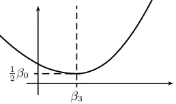
Figure 3: Theσ2 _{function forβ}

0 = 1/2,β1= 1, β2 = 1/2 and β3 = 1,.

The volatility function is defined as

σ2(d) =

(₁

2max(σmin2 +αr(d−d0)2,2σ2M ax), ifd≥d0

1

2max(σmin2 +αl(d−d0)2,2σ2M ax), ifd < d0.

(5.1)

An example ofσ is shown in Figure 3. Overall, the number of parameters to be calibrated isK+ 5:

σ2

min,αl,αr,d0 to specify the volatility functionσ, and α0, α1, . . . , αK to specify the weightϕ.

We use the approach proposed in [13] which allows to price options of different strikes and different times-to-expiration by a single numerical solution of the Cauchy problem (4.2)-(4.3).

The Hobson&Rogers model used in the comparison is defined by the SDEs (2.1) and (2.2) where

σ is specified in (5.1).

In the LV model, St is solution of the SDE

dSt=µtStdt+σ(St, t)StdWt. (5.2)

As shown by Dupire [11], the LV functionσ(St, t) can be directly computed by knowing the option

price as a function of strike and maturity. The number of parameters we have used is equal to the number of option prices in the cross section.

In the stochastic volatility model by Heston, St and σt2, the price and the squared volatility

processes, respectively, are given, in the risk neutral measure, by the solution of the SDE

dSt=rtStdt+σtStdWˆt (5.3)

dσ2_t =κ(σ∞2 −σ

2

t)dt+γσt(ρdWˆt+

p

1₋ρ2_dWˆˆ

t) (5.4)

wheredWˆtanddWˆˆtare two independent Brownian motions on the risk-neutral probability measure.

and Madan which uses a Fourier inversion technique [15, 5]. In the experiments, the σ∞, the

long-term volatility, κ, the mean reversion speed, γ, the volatility of volatility, and ρ, the correlation,

are inferred from market prices.

5.1 Empirical results

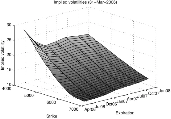
The dataset consists in closing prices of options on futures on the FTSE-100 index quoted at Euronext in the period March 22 – May 19, 2006 and maturities on June, September, December 2006 and March, June, September and December 2007. For each day and each maturity the dataset contains the underlying future price (with values in the range [5675,6307]), the Call and Put closing prices for strikes 4025–6725 and the corresponding implied volatilities. The underlying values have been corrected for dividends, in order to have a common underlying for all the expirations and then option prices are recomputed by using the dataset’s implied volatilities. Thus, after the adjustment the underlying has a null drift in the equivalent martingale measure, that is the interest and dividend rates are null. An example of the implied volatility surface is shown in Figure 4

4000

5000

6000

7000 Apr06Jul06

Oct06Jan07 Apr07Jul07

Oct07Jan08 10

15 20 25 30

Expiration Implied volatilities (31−Mar−2006)

Strike

Implied volatility

Figure 4: Implied Volatility surface for March 31, 2006.

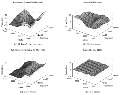
In the first set of experiments, the parameters of the four models are daily calibrated to market prices by a least squares fitting of market prices as in [10, 13]. An example of the absolute pricing errors of the four models on a specific date is reported in Figure 5.

A resume of the performances on each are reported in Figures 6 and 7. These figures plot for each day and for each model the Residual Mean Squared Errors (RMSE) and Residual Mean Squared percentage errors (RMSPE). In the computation of the RMSPE options with price smaller than 5 have been discarded. As can be seen from Figure 6 the fitting of the LV model is, as expected, always almost perfect; that of standard Hobson&Rogers model is at least twice that of the remaining two models. The Heston model is slightly better than the PDV; however the reverse happen when considering relative errors (cf. Figure 7).

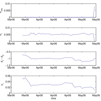
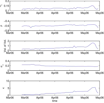
In order to study the stability of the parameters on different samples, their evolution is reported in Figures 8-10 for the Hobson&Rogers, Heston and PDV models. Due to its large number we do not report the evolution of Dupire’s local volatilities, but it is well known they are not stable due to its over-parametrization. The parameters for the Hobson&Rogers model are quite stable until

near the end of the sample, where the model flattens to standard Black and Scholes, αl, αr ≃ 0.

4000 5000 6000 7000 Nov06 Jun07 Dec07 −40 −20 0 20 40 Expiration Hobson and Rogers (31−Mar−2006)

Strike

Pricing Error

(a) Hobson&Rogers errors

4000 5000 6000 7000 Nov06 Jun07 Dec07 −20 0 20 Expiration Heston (31−Mar−2006) Strike Pricing Error

(b) Heston errors

4000 5000 6000 7000 Nov06 Jun07 Dec07 −20 0 20 Expiration Path Dependent Volatility (31−Mar−2006)

Strike

Pricing Error

(c) PDV errors

4000 5000 6000 7000 Nov06 Jun07 Dec07 −20 0 20 Expiration Dupire (31−Mar−2006) Strike Pricing Error

(d) LV’s errors

Figure 5: Pricing error surfaces for Hobson&Rogers, Heston, PDV and Dupire models on March 31, 2006.

Value of the underlying is 5964.5.

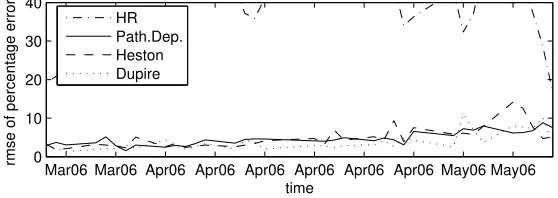
Mar06 Mar06 Apr06 Apr06 Apr06 Apr06 Apr06 Apr06 May06 May06 0 10 20 30 time rmse HR Path.Dep. Heston Dupire

Mar06 Mar06 Apr06 Apr06 Apr06 Apr06 Apr06 Apr06 May06 May06 0

10 20 30 40

time

rmse of percentage errors

HR Path.Dep. Heston Dupire

Figure 7: Root Mean Square of Percentage Errors in pricing.

These two models show spikes in the series of parameters on the same day (cf. the graph of ρ in

Figure 9 and of αr in Figure 10).

This behaviour of the three models can be explained by looking at the time series of the underlying index which is shown in Figure 11. Near the end of the sample, exactly on May 12, the index level drops significantly: consequently the option market reacts and the parameters of the three models try to adapt to market movements.

As a final (and more significant) experiment we compared the hedging performances of the methods by considering the tracking error of the replicating portfolio suggested by each model w.r.t. the evolution of each single call.

For each model we proceed as follows. At the ith day, time ti, the model has been calibrated

to the market cross-section of prices. Then, for a given expiry T and a given strike K we consider

the portfolio composed by a short position on one CallCti and a long on the replicating portfolio

Vti =αiSti+βiBti as in (3.3). That is, the portfolio Πti =Vti−Cti, which has null value in case of

perfect replication. Then, the next day the portfolio has value given byαiSti+1 +βiBti+1−Cti+1,

the corresponding profit and losses are accumulated and a new portfolio Πti+1 is built. Recalling

that we are working on a dividend and interest rate free setting, the total profits and losses on the

period [t1, tn] are given by C1−Cn+Pn

−₁

i=1 αi(Sti+1−Sti).

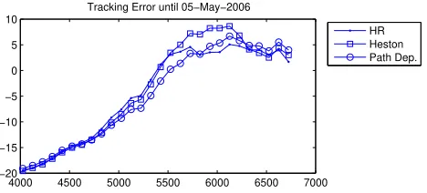
This procedure has been repeated for each model, for each strike, for the expirations June 16, 2006 and December 15, 2006 and for the periods March 22 - May 5 and March 22 - May 19. The two periods correspond to quiet and nervous market situations, respectively (see Figure 11). These performance results are reported on Figures 12-15. Standard delta-hedging have been used for HR and PDV models, while minimum-variance hedging is used for Heston stochastic volatility model [1].

Figure 12 shows the replication error of the hedging strategies until about one month to expi-ration and after the fall of May 12. The HR model is the better for at-the-money options and the Heston model is superior for out-of-the-money options. The PDV model is between the two, but in both the cases is near to the best and the overall performance is thus preferable to the other two. The performances in a quiet market scenario reported in Figure 13 are a bit mixed. In this experiment the overall performances of Heston are slightly better than those of PDV and HR models.

Mar060 Mar06 Apr06 Apr06 Apr06 May06 May06 0.005

0.01

σ min

Mar060 Mar06 Apr06 Apr06 Apr06 May06 May06 0.005

0.01

α l

Mar06 Mar06 Apr06 Apr06 Apr06 May06 May06 −1.5

−1 −0.5

d t

− d

0

Mar060 Mar06 Apr06 Apr06 Apr06 May06 May06 0.02

0.04 0.06

α r

time

Figure 8: Evolution of parameters for HR model, with daily calibration on the test period (March 22 – May

Mar06 Mar06 Apr06 Apr06 Apr06 May06 May06 0.1

0.15 0.2

σ t

Mar06 Mar06 Apr06 Apr06 Apr06 May06 May06

−0.8 −0.6 −0.4

ρ

Mar060 Mar06 Apr06 Apr06 Apr06 May06 May06

1 2

Vol. of Vol.

Mar060 Mar06 Apr06 Apr06 Apr06 May06 May06

0.2 0.4

σ ∞

Mar060 Mar06 Apr06 Apr06 Apr06 May06 May06

5 10

κ

time

Mar060 Mar06 Apr06 Apr06 Apr06 May06 May06 2

4x 10

−3

σ min

Mar060 Mar06 Apr06 Apr06 Apr06 May06 May06

0.5 1

α l

Mar060 Mar06 Apr06 Apr06 Apr06 May06 May06

0.5 1

d t

− d

0

Mar060 Mar06 Apr06 Apr06 Apr06 May06 May06

0.1 0.2

α r

Mar060 Mar06 Apr06 Apr06 Apr06 May06 May06

20 40

a i

time

Figure 10: Evolution of parameters for the PDV model, with daily calibration on the test period.

Apr06 May06

5700 5800 5900 6000 6100

4000 4500 5000 5500 6000 6500 7000 −80

−60 −40 −20 0 20

Tracking Error until 19−May−2006

HR Heston Path Dep.

Figure 12: Hedging error against strike for maturity June 16, 2006. The errors are computed on the period

March 22 - May 19, 2006.

4000 4500 5000 5500 6000 6500 7000 −20

−15 −10 −5 0 5 10

Tracking Error until 05−May−2006

HR Heston Path Dep.

Figure 13: Hedging error against strike for maturity date June 16, 2006. The errors are computed on the

period March 22 - May 5, 2006.

4000 4500 5000 5500 6000 6500 7000 −80

−60 −40 −20 0

Tracking Error until 19−May−2006

HR Heston Path Dep.

Figure 14: Hedging error against strike for maturity December 15, 2006. The errors are computed on the

periodt March 22 - May 19, 2006.

4000 4500 5000 5500 6000 6500 7000 −20

−15 −10 −5 0 5 10

Tracking Error until 05−May−2006

HR Heston Path Dep.

Figure 15: Hedging error against strike for maturity December 15, 2006. The errors are computed on the

References

[1] C. Alexander and L. Nogueira,Hedging options with scale-invariant models, tech. report,

ICMA Centre, University of REading, June 2006.

[2] E. Barucci, S. Polidoro, and V. Vespri, Some results on partial differential equations

and Asian options, Math. Models Methods Appl. Sci., 11 (2001), pp. 475–497.

[3] F. Black and M. Scholes, The pricing of options and corporate liabilities, J. Political

Economy, 81 (1973), pp. 637–654.

[4] V. Blaka Hallulli and T. Vargiolu, Financial models with dependence on the past: a

survey, Applied and Industrial Mathematics in Italy, M. Primicerio, R. Spigler, V. Valente, editors, Series on Advances in Mathematics for Applied Sciences, World Scientific 2005, 69 (2005).

[5] P. Carr and D. Madan,Option pricing and the fast fourier transform, Journal of

Compu-tational Finance, 2 (1999), pp. 61–73.

[6] C. Chiarella and K. Kwon,A complete Markovian stochastic volatility model in the HJM

framework, Asia-Pacific Financial Markets, 7 (2000), pp. 293–304.

[7] R. Cont, Model uncertainty and its impact on the pricing of derivative instruments, Math.

Finance, 16 (2006), pp. 519–547.

[8] M. Di Francesco and A. Pascucci, On the complete model with stochastic volatility by

Hobson and Rogers, Proc. R. Soc. Lond. Ser. A Math. Phys. Eng. Sci., 460 (2004), pp. 3327– 3338.

[9] , On a class of degenerate parabolic equations of Kolmogorov type, AMRX Appl. Math. Res. Express, (2005), pp. 77–116.

[10] B. Dumas, J. Fleming, and R. E. Whaley, Implied volatility functions: empirical tests,

J. Finance, 53 (1998), pp. 2059–2106.

[11] B. Dupire, Pricing and hedging with smiles, in Mathematics of derivative securities

(Cam-bridge, 1995), vol. 15 of Publ. Newton Inst., Cambridge Univ. Press, Cam(Cam-bridge, 1997, pp. 103– 111.

[12] G. Fig`a-Talamanca and M. L. Guerra,Complete models with stochastic volatility: further

implications, Working Paper, Universit`a della Tuscia, Facolt`a di Economia, 5 (2000).

[13] P. Foschi and A. Pascucci, Calibration of the Hobson&Rogers model: empirical tests.,

Preprint AMS Acta, University of Bologna, (2005).

[14] M. Hahn, W. Putsch¨ogl, and J. Sass,Portfolio optimization with non-constant volatility

and partial information, preprint, (2006).

[15] S. Heston, A closed-form solution for options with stochastic volatility with applications to

bond and currency options., Review of Financial Studies, 6 (1993), pp. 327–343.

[16] D. G. Hobson and L. C. G. Rogers, Complete models with stochastic volatility, Math.

[17] L. H¨ormander, Hypoelliptic second order differential equations, Acta Math., 119 (1967), pp. 147–171.

[18] F. Hubalek, J. Teichmann, and R. Tompkins, Flexible complete models with stochastic

volatility generalising Hobson-Rogers, working paper, (2004).

[19] R. C. Merton,Theory of rational option pricing, Bell J. Econom. and Management Sci., 4

(1973), pp. 141–183.

[20] A. Platania and L. C. G. Rogers,Putting the Hobson&Rogers model to the test, working

paper, (2006).

[21] S. Polidoro, Uniqueness and representation theorems for solutions of