An Iterative Method for Solving Two Special Cases of Lane Emden Type Equation

(1)

http://dx.doi.org/10.4236/ajcm.2014.43021

An Iterative Method for Solving Two Special

Cases of Lane-Emden Type Equation

Pedro Pablo Cárdenas Alzate

Department of Mathematics, Universidad Tecnológica de Pereira, Pereira R, Colombia Email: [email protected]

Received 18 March 2014; revised 22 April 2014; accepted 8 May 2014

This work is licensed under the Creative Commons Attribution International License (CC BY). http://creativecommons.org/licenses/by/4.0/

Abstract

In this work we apply the differential transformation method or DTM for solving some classes of Lane-Emden type equations as a model for the dimensionless density distribution in an isothermal gas sphere y 2y e y 0

x

±

 _′′₊ _′₊ ₌ 

 

  and as a study of the gravitational potential of (white-dwarf) stars

(

)

3 2

2

0

2

y y y C

x −

 _′′₊ _′₊ ₌ 

 

 , which are nonlinear ordinary differential equations on the semi-in-

finite domain [1] [2]. The efficiency of the DTM is illustrated by investigating the convergence results for this type of the Lane-Emden equations. The numerical results show the reliability and accuracy of this method.

Keywords

Differential Transformation, Lane-Emden, Isothermal Gas Sphere, White-Dwarfs, Iterative Method

1. Introduction

Other classical nonlinear equation, which has been the object of much study, is Lane-Emden’s equation. This equation has the form

( )

2

0

y y g y

x

′′+ ′+ = (1) with 0< ≤x 1 and the subject to initial conditions

( )

0 ,

( )

0

(2)

where α and β are constants and g y

( )

is a real-valued continuous function where α and β are con-stants and g y

( )

is a real-valued continuous function. The Equation (1) was used to model various problems, including the isothermal gas spheres, theory of thermionic currents and the gravitational potential of stars [1] among others.

Let us consider a spherical cloud of gas (see Figure 1) and denote its hydrostatic pressure at a distance r1

from the centre by P. Let M r

( )

1 be the mass of the spheres of radius r1,φ the gravitational potential of the

gas and g the acceleration of gravity. Then, we have the following equation

( )

_{( )}

2 1

1

1 GM r

g r

r φ′

= = − (3)

where G is the gravitational constant.

Thus, three conditions are assumed for the determination of φ and P

1

dP= −gρdr =ρ φd (4)

where ρ is the density of the gas.

( )

2

1 1

1

2

4π

r r G

r ρ

φ φ′′ φ′

∇ = + = − (5)

and

P=Kργ (6)

where γ and K are arbitrary constants.

Now, solving (4) and (6) with φ=0 when ρ=0 we have

1 1

1 1 K

γ γ

ρ φ₌ − −

(7)

or

n

L

ρ= φ (8)

where 1

1

n

γ =

− and

n

L=K− . If this value of ρ is replaced into Equation (5), we obtain

2φ δ φ2 n

∇ = − (9)

where δ =2 4πLG.

(3)

Now, since 1dP dφ

ρ = , by integration 0

log

K ρ

φ

ρ  

= _ _

 , that is, 0e K

φ

ρ ρ= . If ρ0 is the central density,

then φ0 must be zero, a change from the condition in the previous case where φ was zero only at the

boun-dary of the sphere.

Poisson’s equation is now replaced by

2 2_eK

φ

φ δ

∇ = − (10) where δ2 =4πρ0G, equation which is known as Liouville’s equation. If we assume symmetry as before,

Equa-tion (1) in polar coordinates reduces to the following

( )

2

1 1

1

2

eK 0

r r

r

φ

φ′′ + φ′ +δ = (11)

which replaces Equation (9).

If we let φ =Ky and 1 K

r x

δ

= , then (11) becomes

2

ey 0

y y

x

′′+ ′+ = (12) which is to solved subject to the boundary conditions y

( )

0 =0 and y′

( )

0 =0. The counterpart [2] of the Eq-uation (12) in which ey is replaced by e−y appears in Richardson’s theory of thermionic currents when one seeks to determine the density and electric force of an electron gas in the neighborhood of a hot body in thermal equilibrium.

Finally, now consider g y

( )

=

(

y2−C

)

3 2, then Equation (1) is turned to the white-dwarf equation, which introduced by [2] in his study of gravitational potential of the degenerate stars. This Equation is defined in the form

(

₂

)

3 2 2

0

y y y C

x

′′+ ′+ − =

With x∈

[ ]

0,∞ and subject to initial conditions y

( )

0 =1 and y′

( )

0 =0. For instance if C=0, we have Lane-Emden equation of index m=3 [3].

The Differential Transformation Method is a semi-numerical-analytic method for solving ordinary and partial differential equations. Zhou first introduced the concept of DTM in 1986 [4]. This technique constructs an ana-lytical solution in the form of a polynomial. DTM is an alternative procedure for obtaining anaana-lytical Taylor se-ries solution of the differential equations. The sese-ries often coincides with the Taylor expansion of the true solu-tion at point x0=0, in the value case, although the series can be rapidly convergent in a very small region.

Many numerical methods were developed for this type of nonlinear ordinary differential equations, specifi-cally on Lane-Emden type equations such as the Adomian Decomposition Method (ADM) [5], the Homotopy Perturbation Method (HPM) [6] [7], the Homotopy Analysis Method (HAM) [8] and Berstein Operational Ma-trix of Integration [9]. In this paper, we show superiority of DTM by applying them on the some type Lane- Emden type equations. The power series solution of the reduced equation transforms into an approximate impli-cit solution of the original equation. A spectral method (Legendre-Spectral method) was proposed to solve white-dwarf equation; this spectral method provides the most convenient computer implementation [10].

2. Description of DTM

Differential transformation method of the function y x

( )

is defined as follows

( )

0 d

1

! d

k

k x x

y x Y k

k x ₌

 

=  

 

  (13)

(4)

transformation is defined by

( )

₀

( )

k k

y x =

∑

∞₌ Y k x (14)

In real applications, function y x

( )

is expressed by a finite series and Equation (14) can be written as

( )

0

n k

k= Y k x

∑

(15) Equation (15) implies that

( )

1

k

k n

Y k x

∞

= +

∑

The following theorems can be deduced from Equations (13) and (15).

Theorem 1 If theny x

( )

= f x

( )

±g x

( )

, Y k

( )

=F k

( )

±G k

( )

.

Theorem 2 If they x

( )

=af x

( )

, , n Y k

( )

=aF k

( )

a∈.

Theorem 3 If then

( )

d

( )

,

( ) (

) ( )

! !

d

n

g x k n

y x Y k G k n

k x

+

= = + .

Theorem 4

( )

( ) ( )

( )

( ) (

)

1 0 1 1 ,

If then k

k

y x =g x h x Y k =

∑

₌ G k H k−k .

Theorem 5

( )

, , where

( )

(

)

(

)

1, 0,

If then n k n

y x x Y k k n k n

k n

δ δ  =

= = − − =  _≠



Theorem 6 (Cárdenas) I

( )

, with , then

( )

0,

₍

₎

,

f y x x f xn m N Y k k m

F k m k n

< 

= ∈ _{= }

− ≥

 The proofs of Theorems are available in [11].

3. Test Problems

To illustrate the ability of DTM for the Lane-Emden type equation, three examples are provided. The results re-veal that this method is very effective.

Example 1 Consider the nonlinear initial-value problem y 2y ey 0

x

′′+ ′+ = subject to y

( )

0 =y′

( )

0 =0. Multiplying both sides by x we obtain

2 ey 0

xy′′+ y′+x = (16) Applying theorems 1-6 to Equation (16)

(

_{) ( )( ) ( ) ( )}

1 2 3

1 1 1 1

1 1 1

2 1 2! 3! 4!

Y k k Y k S S S

k k δ

−  

+ = _ − + − + + + + _

+ +   (17)

where

( ) (

)

1

1 0

1 1 1

k

S Y k Y k k

−

=

∑

− − (18)

( ) (

) (

)

2

2 1

1

2 1 2 1 0

2 0

1 k k

k k

S Y k Y k k Y k k

− = =

=

∑

− − − (19)

( ) (

) (

)

3 2

3 2 1

1

3 1 2 1 3 2 3

0 0 0

1 k k

k

k k k

S Y k Y k k Y k k Y k k

−

= = =

=

∑ ∑ ∑

− − − − (20)

for all k≥1.

Now, from the initial conditions y

( )

0 = y′

( )

0 =0 we can obtain

( )

0 0 and

( )

1 0

Y = Y = (21)

(5)

( )

1

(

)

( )

1

1, 2 1 1 0 0 0

For

6 6

k= Y =− _δ − +Y + + _=− .

( )

(

) ( )

( ) (

)

( ) (

) (

)

2 2 1 1 1 1 1

1 2 2

0 1 0 1 0 1 1

2, 3 2 1 1 1

12 2! 1 1 o 3 r ! F 0 k k k k

k Y Y Y k Y k k

Y k Y k k Y k k

δ = = =  − = = _ − + + − −   − − − _{+ }  +

∑ ∑

=

∑



and then, Y

( )

3 =0. For k=3 we have:

( )

(

) ( )

1 2 3

1 1 1 1

4 3 1 2

5 4 2! 3! 4!

Y = − _δ − +Y + S + S + S + _

×  

Now, as

( )

2 1 6

Y =− and S1=S2=S3==0, then

( )

1 1

4

4 5 6 120

Y = =

× ×

For k=4 we have:

( )

(

) ( )

1 2 3

1 1 1 1

5 4 1 3

6 5 2! 3! 4!

Y = − _δ − +Y + S + S + S + _

×  

In this case as Y

( )

3 =0 and S1=S2=S3==0, then Y

( )

5 =0.

The lector can see that

( ) (

)

( ) ( )

1

3

1 1 1

0

1 0 3 1 2 2 1 3 0 0

k

S Y k Y k k Y Y Y Y Y Y Y Y

=

∑

− − = + + + =

For k=5 we have:

( )

(

)

( )

1 2 3

1 1 1 1

6 5 1 4

7 6 2! 3! 4!

1 1 1 1 1

7 6 120 2! 3! 4!

Y Y S S S

S S S

δ −   = _ − + + + + + _ ×     = − _ + + + + _ ×    

Now, we can see:

( ) (

)

( ) ( )

1

4

1 1 1

0

1 0 4 1 3 2 2 3 1 4 0

1 1 1

6 6 36

k

S Y k Y k k Y Y Y Y Y Y Y Y Y Y

=

= − − = + + + +

−

= × − =

∑

2 3 0

S =S == and then

( )

1 1 1 1 8

6

7 6 120 2! 36 21 6!

Y = − _ + × _= −

×   ×

For k=6 we have:

( )

(

)

( )

1 2 3

1 1 1 1

7 6 1 5

8 7 2! 3! 4!

1 1 1 1

8 7 2! 3! 4!

Y Y S S S

S S S

δ −   = _ − + + + + + _ ×     = − _ + + + _ ×     Here,

( ) (

)

( ) ( )

1 0 1 5

1 1 1 0 5 1 4

2 3 3 2 4 1 5 0 0

k

S Y k Y k k Y Y Y Y

Y Y Y Y Y Y Y Y

=

= − − = + +

+ + + =

(6)

and

( ) (

) (

)

2

2 1

2 1 2 1

5

0 0

2

1 0

k

k k

= =

=

∑ ∑

− − − =

and so, S2=S3==0. Consequently, Y

( )

7 =0.

For k=7 we have:

( )

(

)

( )

1 2 3

1 1 1 1

8 7 1 6

9 8 2! 3! 4!

1 8 1 1 1

9 8 21 6! 2! 3! 4!

Y Y S S S

S S S

δ

−  

= _ − + + + + + _

×  

−

 

− _ + + + + _

×  × 



Here

( ) (

)

( ) ( )

1

6

1 0

1 1 1 0 6 1 5 2 4

1 1 1 1 1

3 3 4 2 5 1 6 0

6 120 120 6 360

k

S Y k Y k k Y Y Y Y Y Y

Y Y Y Y Y Y Y Y

=

= − − = + +

− −

+ + + + = × + × − =

∑

and

( ) (

) (

)

2

2 1

6

0

2 1 2 1 2

0

1 1

216

k

k k

= =

−

=

∑ ∑

− − − =

Consequently, S3=S4==0. Finally,

( )

1 8 1 1 1 1 61

8

9 8 21 6! 2 360 6 216 1632960

Y = −  −_ + × −_ _+ × −_ __=

×  ×    

Therefore using (15), the closed form of the solution can be easily written as:

( )

0

( )

1

( )

2

( )

3

( )

4

0

2 4 6 8

0 1 2 3 4

1 1 1 61

6 120 21 6! 1632960

n

k

y x Y k x Y x Y x Y x Y x Y x

x x x x

=

= = + + + + +

= − + − + − ×

∑



A series solution obtained by Wazwaz [5] and series expansion respectively is

( )

1 2 1 4 1 6 122 8 61 67 10

6 5 4! 21 6! 81 8! 495 10!

y x ≅ − x + x − x + x − × x +

× × × ×  (22)

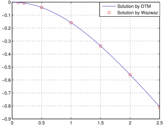
Table 1shows the comparison of y x

( )

obtained by the DTM (method proposed in this work) and those ob-tained by Wazwaz. The resulting graph of the isothermal gas spheres equation in comparison to the present me-thod and those obtained by Wazwaz is shown in Figure 2.

Example 2 Consider the following problem y 2y e y 0

x

−

′′+ ′+ = subject to y

( )

0 =y′

( )

0 =0. Multiplying both sides by x

2 e y 0

xy′′+ y′+x − = (23)

As before, using theorems 1-6 we obtain

(

_{) ( )( ) ( ) ( )}

1 2 3

1 1 1 1

1 1 1

2 1 2! 3! 4!

Y k k Y k S S S

k k δ

−  

+ = _ − − − + − + − _

+ +   (24)

where S S1, 2 and S3 are as (18), (19) and (20) respectively for all k≥1. Now, from the initial conditions

( )

0

( )

0 0

y =y′ = we have

( )

0 0 and

( )

1 0

[image:6.595.87.486.94.507.2]

(7)

[image:7.595.178.447.89.301.2]

Figure 2. Comparison between DTM and Wazwaz’s algorithm.

Table 1. Comparison between DTM and Wazwaz’s algorithm.

𝒙𝒙 DTM Wazwaz Error

0.0 0.0000000000 0.0000000000 0.0000000000

0.1 −0.0016658338 −0.0016658338 0.0000000000

0.2 −0.0066533671 −0.0066533671 0.0000000000

0.5 −0.0411539573 −0.0411539568 0.0000000005

1.0 −0.1588276775 −0.1588273536 0.0000003239

1.5 −0.3380194248 −0.3380131102 0.0000063146

2.0 −0.5598230174 −0.5599626601 0.0001396427

2.5 −0.8063552923 −0.8100196713 0.0036643790

Substituting Equation (25) into Equation (24) and by recursive method, the results are listed as follows. For k=1, 2,3, 4,5, we have respectively

( )

1

( )

1

( )

1

2 , 3 0, 4 , 5 0, 6

6 120 1890

Y = − Y = Y = − Y = Y = −

So on, we can use (15) and the closed form of the solution can be easily written as

( )

0

( )

1

( )

2

( )

3

( )

4

0

2 4 6

0 1 2 3 4

1 1 1

6 120 1890

n

k

y x Y k x Y x Y x Y x Y x Y x

x x x

=

= = + + + + +

= − − − −

∑



A solution obtained by Yahya [12] by using the power series method is

( )

1 2 1 4 8 6 122 8

6 120 21 6! 81 8!

y x ≅ − x − x − x − x −

× × 

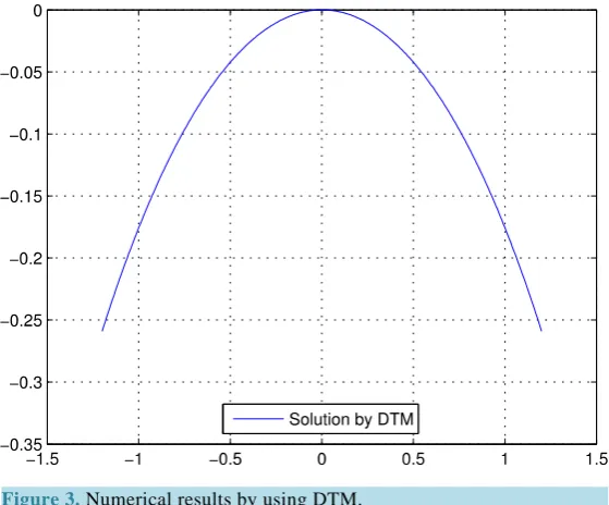
We can see Figure 3and compare with [13], the results are very good.

[image:7.595.88.537.336.495.2]

(8)

[image:8.595.173.453.85.317.2]

Figure 3. Numerical results by using DTM.

Example 3 Consider the problem _y 2_y

(

_y2 _c

)

3 2 ₀

x

′′+ ′+ − = subject to y

( )

0 =1 and y′

( )

0 =0. Multiplying both sides by x we obtain

(

₂

)

3 2

2 0

xy′′+ y′+x y −c = (27)

Here, is easy to verify that the function g y

( )

=

(

y2−c

)

3 2 has a series expansion

( )

3

(

)

2

(

)

2 2

(

)

3

3 3 9 3

3 1 1 1

2 3!

q q

g y q q y y y

q q

+ −

≈ + − + − + − + (28)

where q2 = −1 c. Therefore, Equation (27) takes the form

(

)

2

(

)

2 2

(

)

3

3 3 9 3

2 3 1 1 1

2 3!

q q

xy y x q q y y y

q q

 + − 

′′+ ′+ _ + − + − + − + _

  (29)

Using in (29) the above theorems we have the following

(

) (

)

(

)

(

)

3 4

1 2 1 2

1 1 2 1 1 1 1

2! 3!

k+ kY k+ + k+ Y k+ +α δ k− +α Y k− +α S +α S  (30) or

(

_{) ( )( )}

(

)

(

)

3 4

1 2 1 2

1

1 1 1

2 1 2! 3!

Y k k Y k S S

k k

α α

α δ α

 

+ = _− − − − − − _

+ _{+ } _ (31)

where

2 2

3

1 3

2 2

2 3

2 2

3 3

3 3 9 3

3

2 3!

3 3 9 3

3 2 3

2 3!

3 3 9 3

3

2 3!

q q

q

q q

α

+ −

= − + − +

+ −

= − + +

+ −

= − +



(9)

and successively. Also,

( ) (

)

1

1 k 0 1 1 1

k

S =

∑

−₌ Y k Y k− −k (32)

( ) (

) (

)

2 2 1

2 1 2 1

1

0 k 0 1 2

k k k

S =

∑

−₌

∑

₌ Y k Y k −k Y k− −k (33)

( ) (

) (

)

3 2 3 2 1

3 1 2 1 3 2

1

0 0 0 1 3

k k k

S =

∑ ∑ ∑

−₌ ₌ ₌ Y k Y k −k Y k −k Y k− −k (34)

for all k≥1. Now, from the initial conditions we have

( )

0 1 and

( )

1 0

Y = Y = (35)

Substituting (35) into Equation (31) and by recursive method, the results are listed as follows.

For

( )

3 3

1 2

1 1

1, 2

6 2! 6

k= Y = _− −α α −α _= − q

  . or

( )

(

)

( )

3

1 2 1

1

2, 3 2 1 1 0

12 2!

k= Y = _−α δ − −α Y −α S − _=

 

and then

( )

(

)

( )

3

1 2 1

1

3 0. 3, 4 3 1 2

20 2!

for

Y = k= Y = _−α δ − −α Y −α S − _

  and then

( )

4 1 4

40

Y = q . For

( )

(

)

( )

3

1 2 1

1

4, 5 4 1 3

30 2!

k= Y = _−α δ − −α Y −α S − _

  and so Y

( )

5 =0. For

( )

(

)

( )

3

1 2 1

1

5, 6 5 1 4

42 2!

k= Y = _−α δ − −α Y −α S − _

  therefore

( )

7 5

5 14

6

5040 5040

Y = − q − q . Using (15), the

closed form of the soluyion can be easily written as

( )

(

)

(

)

(

)

(

)

0 2 3

0

3 2 2 4 4 7 2 5 2 6

( ) 0 1 2 3

1 1 5 14

1 1 1 1 1 .

6 40 5040 5040

n

k

y x Y k x Y x Y x Y x Y x

c x c x c c x

=

= = + + + +

 

= − − + − −_ − + − _ +

 

∑



A series solution obtained by Chandrasekhar [2] using series expansion was

( )

3 2 4 4 5

(

2

)

6 6

(

2

)

8

1 5 14 339 280

6 40 7! 3 9!

q q q q

y x ≅ − x + x − q + x + q + x +

×  (36)

Table 2 shows the comparison of y x

( )

obtained by the DTM and those obtained by Parand [14]. The re-sulting graph of the white-dwarfs equation in comparison to the present method and the obtained by [14] is show inFigure 4.

4. On Convergence of DTM

[image:9.595.89.539.575.724.2]

We can write the DTM as

Table 2. Comparison between DTM and Legendre-Spectral method. x DTM L-S method Error

0.0 0.0000000000 0.0000000000 0.0000000000

0.5 0.9812035800 0.912034800 0.0000001000

1.0 0.9270041568 0.9270031568 0.0000010000

1.5 0.8439248841 0.8439247581 0.0000001260

2.0 0.7425430743 0.7425430235 0.0000000508

2.5 0.6365969111 0.6365953025 0.0000016086

3.0 0.5410635754 0.5410633690 0.0000002064

(10)

Figure 4. Comparison between DTM and a Legendre-Spectral Method.

(

1

)

0 , , , ; , 0, ,

k

j n j f n n n k

j= α y+ =hφ x y y+ − h n= N−k

∑

  (37)

where φ_f increase function depends on its arguments through the function f . The method (37) means k

steps, needed for early values k y: n,,yn k+ −1 to calculate yn k+ . It is therefore necessary to have bootstrap

values y0,,yk−1.

The method (37) is said to be convergent if for all IVP has to

(

)

(

)

0 1

lim max _n _n 0 if lim max _n _n 0

N→∞k n N≤ ≤ y x −y = N→∞ ≤ ≤ −n k y x −y =

Remark. The condition

(

)

0 1

lim max _n _n 0

N n k

y x y

→∞ ≤ ≤ − − = on the bootstrap values is equivalent to asking that

( )

0 0

lim n h

y y x

+

→ = for n=0,,k−1. Here, we are asking that bootstrap values

{ }

1 0 k n n

y −₌ approximate well and

the initial data y x

( )

0 ; if this is not, then no reason to expect that numerical solution closely matches the

theo-retical.

Now let us consider the following form of the Equation (1)

( )

(

)

y x =0₍₃₈₎ Here is a nonlinear differential operator, which encloses the linear and nonlinear term of the Lane-Emden

type equation. Now, the linear term = y( )n _{is always invertible and the nonlinear term is Therefore (38)}

may be written as

( )

(

)

(

( )

)

y x + y x =0₍₃₉₎

or

( )

(

)

(

( )

)

y x = − y x =0₍₄₀₎ Applying DTM in (40) we can obtain

(

k+1

)(

k+2

) (

 k+n Y k

) (

+n

)

= −

(

y x

( )

)

(41) Remember that differential transformation of _{and are computed by using theorems 1 - 6.}

Let us consider the Equation (38) in the following form

( )

(

( )

)

(11)

Here, is a nonlinear operator. It is noted that Equation (15) is equivalent to the sequence

( )

0 1 2

0

n k

n n

k= Y k x =y +y +y + +y =T

∑

 (43)

This sequence is determined using the iterative scheme

( )

1

n n

T₊ = T ₍₄₄₎

and associated with T =

( )

T .

The following theorem guarantees that the scheme of DTM converges to the solution y x

( )

of Lane-Emden Equation (1).

Theorem 7 Let be a nonlinear operator from a Banach space and y x be the solution

( )

(exact) of Equation (42). The series solution (14) converges to y x

( )

, if there exists a constant 0≤ <c 1 such that

1

k k

y₊ ≤c y for k∈+

{ }

0 .

Proof. We prove that the sequence

{ }

Tn n ₀

∞

= is a Cauchy sequence in . Therefore,

2 1

1 1 1 0

n

n n n n n

T −T+ = y+ ≤c y ≤c y− ≤≤c + y

Thus, for any m n, ∈+,m≤n,

(

)

1 1 2 1

1 1

0 0 0

1 2

0

1

0

1 1

n m n n n n m n

n n m

m m n

n m m

T T T T T T T T

c y c y c y

c c c y

c

c y

c

− − − +

− +

+ +

− +

− ≤ − + − + +

=

− ≤ + + +

≤ + + + −

−

  

so

1

0

1

m

n m

c

T T y

c

+

− <

− implying that he sequence

{ }

Tn n 0

∞

= is Cauchy, i.e. since 0≤ <c 1 then

,

lim n m 0

n m→∞ T −T = , therefore there exists T∈ such that limn→∞Tn=T, i.e. T n 0yn

∞ =

=

∑

converges.

Now, we can say too that Equation (42) is similar to solve T =

( )

T , therefore this implies that if is con-tinuous then

( )

(

)

( )

(

1

)

lim _n lim _n lim _n

n n n

T T T T₊ T

→∞ →∞ →∞

= = = =

[image:11.595.212.424.528.699.2]

i.e.T is a solution of y x

( )

=

(

y x

( )

)

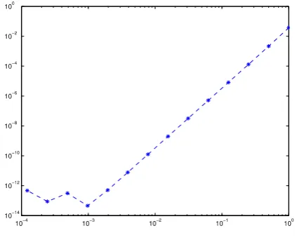
and this completes the proof.

Figure 5shows the maximum point-wise error between the numerical solution obtained by using DTM and the Chandrasekhar solution. It is observed that both schemes are almost the same accuracy.

(12)

5. Conclusion

In this work, we presented the definition and handling of one-dimensional differential transformation method. Using DTM, the Lane-Emden equations were transformed into algebraic equations (iterative equations). The new scheme obtained by using DTM yields an analytical solution in the form of a rapidly convergent series. This me-thod makes the solution procedure much more attractive. The figures and tables clearly show the high efficiency of DTM and the convergence of the method for three examples in investigated.

Acknowledgements

Foremost, I would like to express my sincere gratitude to Jean-Christophe Nave (Department of Mathemat-ics and StatMathemat-ics McGill University) for the support of my research and the support of the Department of Ma-thematics of the Universidad Tecnológica de Pereira (Colombia) and the group GEDNOL.

References

[1] Davis, H. (1962) Introduction to Nonlinear Differential and Integral Equations. Dover, New York. [2] Chandrasekhar, S. (1967) Introduction to Study of Stellar Structure. Dover, New York.

[3] Liao, S.J. (2003) A New Analytic Algorithm of Lane-Emden Type Equations. Advances in Applied Mathematics, 142, 1-16. http://dx.doi.org/10.1016/S0096-3003(02)00943-8

[4] Zhou, J.K. (1986) Differential Transformation and Its Applications for Electrical Circuits. Huazhong University Press, Wuhan.

[5] Wazwaz, A.M. (2001) A New Algorithm for Solving Differential Equations of Lane-Emden Type. Applied Mathemat-ics and Computation, 118, 287-310. http://dx.doi.org/10.1016/S0096-3003(99)00223-4

[6] Gorder, R.A. (2011) An Elegant Perturbation Solution for the Lane-Emden Equation of the Second Kind. New As-tronomy, 16, 65-67. http://dx.doi.org/10.1016/j.newast.2010.08.005

[7] Ramos, J.I. (2008) Series Approach to the Lane-Emden Equation and Comparison with the Homotopy Perturbation Method. Chaos Solitons Fractals, 38, 400-408. http://dx.doi.org/10.1016/j.chaos.2006.11.018

[8] Iqbal, S. and Javed, A. (2005) Application of Optimal. Advances in Applied Mathematics, 42, 29-48.

[9] Kumar, N. and Pandey, R. (2011) Solution of the Lane-Emden Equation Using the Bernstein Operational Matrix of In-tegration. ISRN Astronomy and Astrophysics, 2011, 1-7. http://dx.doi.org/10.5402/2011/351747

[10] Rismani, A.M. and Monfared, H. (2102) Numerical Solution of Singular IVPs of Lane-Emden Type Using a Modified Legendre-Spectral method. Applied Mathematical Modelling, 36, 4830-4836.

http://dx.doi.org/10.1016/j.apm.2011.12.018

[11] Cárdenas, P. and Arboleda, A. (2012) Resolución de ecuaciones diferenciales no lineales por el método de trans-for-mación diferencial, tesis de maestría en matemáicas. Universidad Tecnológica de Pereira, Colombia.

[12] Yahya, H. (2012) On the Numerical Solution of Lane-Emden Type Equations. Advances in Computational Mathemat-ics and Its Applications (ACMA), 4, 191-199.

[13] Batiha, B. (2009) Numerical Solution of a Class of Singular Second-Order IVPs by Variational Iteration Method. In-ternational Journal of Mathematical Analysis, 3, 1953-1968.

http://www.m-hikari.com/ijma/ijma-password-2009/ijma-password37-40-2009/batihaIJMA37-40-2009.pdf [14] Parand, K. and Hojjati, G. (2011) An Efficient Computational Algorithm for Solving the Nonlinear Lane-Emden Type