Analytical and Numerical Solution of One Dimensional a Rectangular Fin with an Additional Heat Source

(1)

Page 1

Analytical and Numerical Solution of One-Dimensional a Rectangular Fin with an Additional Heat

Source

Saeed J. Almalowi

1

_{Corresponding author, Mechanical Engineering Department, Taibah University, Almadianh Almunwwarah, KSA}

---*---Abstract -**

A rectangular fin with constant fin base

thickness was analyzed by using a numerical and an analytical method. The heat source is added to the fin which provides an additional heat source. It dissipates more heat rate to the surrounding. The uniform cross-section extended surface with heat source was conducted in this paper to get more heat in the surrounding fluid. The second order differential equation was solved analytically for a rectangular fin with uniform cross-section area. The temperature profiles were plotted for various values of parameter (M) either with or without heat source.

Key Words: Fin, Analytical, Homogenous, Efficiency,

Uniform

1. Introduction

The uniform extended surface is investigated in this paper. Several studies investigated 1D non-uniform cross-section fins using approximation solutions. In this study, the exact solution was derived for one example of the non-uniform fin. In the literature, non-uniform sub-elements were considered for FEM (efficient FEM, EFEM) solution to reduce the computational complexity. ShahNor et al. was applied for the solution of one-dimensional heat transfer problem in a rectangular thin fin. The obtained results are compared with CFEM and efficient DQM (EDQM), with non-uniform mesh generation) [1]. Antonio et al. studied in a convincing manner that approximate analytic temperature profiles of good quality are easy to obtain without resorting to the exact analytic temperature profile embodying four modified Bessel functions [2]. The influence of fin base height and fin base thickness on the temperature of a rectangular fin were studied by Hyung S. [3]. S. Sunil et al. investigated the 1D transient thin rectangular fin. They studied the temperature and velocity distributions in the field, the temperature profile in the fin, local Nusselt numbers along the fin and the average heat transfer coefficient of the fin are obtained by solving the governing equations in the field and the heat transfer equation in the fin simultaneously, using an explicit unsteady Finite Difference formulation leading to the steady state result [4]. Lien-Tsai and his collogues

optimized the rectangular fin with variable thermal parameters [5].The performance of rectangular fins under natural convection at different orientation of heat sink was investigated by A.A.Walunj et al. [6]. Numerical solutions for the relevant energy balance equation for a longitudinal fin in dimensionless variables were obtained by C. Harley and R.J. Moitsheki through the implementation of an in-built function, bvp4c, in MATLAB [7]. Raseelo J. Moitsheki and Atish R. studied two-dimensional steady rectangular fin. They assumed that thermal conductivity, internal energy generation function, and heat transfer coefficient are dependent on temperature. They employed the Kirchoff transformation on the governing equation [8]. The interaction of thermal radiation with convection is numerically investigated, and an exact solution is presented for temperature distribution of fin of constant cross -sectional area were investigated by

Masoud A. and his colleagues [9]. A. Moradi employed the differential transformation method (DTM) for thermal characteristics of straight rectangular fin for all type of heat transfer and numerical comparison between DTM and a domain decomposition method (ADM) and exact analytical solution method. He presented a numerical with fourth order Rang- Kutta method using shooting method [10]. A. Campo and I. Lira applied a simple approximate to get analytic solution of the quasi 1-D heat equation for annular fins of variable profile. In their study the annular fin of hyperbolic profile was selected. To solve the governing quasi 1-D heat equation in this annular fin approximately, usage of the mean value theorem for integration from calculus was made [11].

2. Mathematical Model

2.1. Analytical Methodology

Figure 1 illustrates a rectangular, has a thickness (H) that has constant in its value at base to the tip of the fin. The fin is surrounded by the fluid at (T∞ = 22oC) with average

convective heat transfer . The fin material

has thermal conductivity (k =3W/m-k) and the base temperature of the fin is kept at (Tb = 150 oC).The tip of

(2)

Page 2

current .The cross section area of the

straight triangular fin, as shown in Figure 1a, is

Figure1. Geometric diagram of the rectangular fins with heat generation

The governing equation can be derived by applying the energy balance as:

Employing Fourier’s Law on Equation (2) yields:

Applying Newton’s cooling law on the convection terms in Equation (3) yields:

Simplifying Equation (4) yields:

Normalizing Equation (5) by using

Where the convection /conduction ratio can be defined in as

The dimensionless energy source parameter is defined as

Equation (7) becomes

Equation (10) is non-homogenous differential equation, and the general solution is divided into a homogenous and particular solution:

The homogenous part can be defined as:

To obtain the solution of the homogenous part assume an exponential solution as:

The particular solution of Equation (10) is

Substituting into Equation (10) the particular solution becomes

The general solution of non-homogenous differential equation is

T

∞

,

x

H.G

L=0.2m

W=0.1m

H=0.01m

(3)

Page 3

After applying the boundary conditions at X=0, θ(X=0) =θb

Substituting C1 and C2 into Equation (16) leads to:

The fin efficiency is

2.2 Numerical Methodology

1) Using the central discretizing scheme for interior nodes on Equation (11) leads to:

Applying the boundary condition at i=1 and i=Nx leads to:

(24)

Using backward scheme for the right boundary leads to:

The dissipated heat via the fin can be evaluated as:

The fin efficiency is defined as

The temperature profiles along the fin were investigated by using the finite difference method and the analytical solution of the second order differential equation, as shown in Figures 2. Figure 2 shows the temperature distribution of the rectangular fin with additional heat source. The temperature was plotted from the base to the

(4)

Page 4

0 0.1 0.2 0.3 0.4 0.5 0.6 0.7 0.8 0.9 1

0.84 0.86 0.88 0.9 0.92 0.94 0.96 0.98 1 1.02

X

 Exact,M=0.2_{Prediction,M=0.2}

Exact,M=0.6 Prediction,M=0.6

0 0.1 0.2 0.3 0.4 0.5 0.6 0.7 0.8 0.9 1 1

2 3 4 5 6 7

X

 Exact,M=0.2

Prediction,M=0.2 Exact,M=0.6 Prediction,M=0.6

0 0.1 0.2 0.3 0.4 0.5 0.6 0.7 0.8 0.9 1 1

2 3 4 5 6 7

X



M=0.2 M=0.4 M=0.6 M=0.8 M=1.0 0 0.1 0.2 0.3 0.4 0.5 0.6 0.7 0.8 0.9 1 0.2

0.3 0.4 0.5 0.6 0.7 0.8 0.9 1

X



M=0.2 M=0.4 M=0.6 M=0.8 M=1.0

Figure 2.Temperature profiles at various values of M for the rectangular fin with heat source

Figure 3 illustrates the dimensionless temperature distribution as a function of position (X) for various values of parameter (M) when the heat sources parameter ψ =0. Regardless of the value of parameter (M), the solution should satisfy the boundary conditions; the curves intersect at the base of the fin and the slope of each curve is zero at (X=1). However, the shape of the curves changes with M. Smaller values of parameter (M) results in a smaller temperature drop due to conduction along the fin whereas large values of M have a corresponding large temperature drop due to conduction and little for convection. Consequently, M represents the balance of the conduction along the fin and the convection from fin’s surface.

[image:4.595.50.267.86.268.2]

Figure3.Temperature profiles at various vales of M for the rectangular fin without heat source

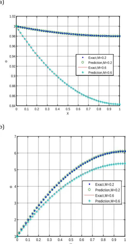
Figure 4 a and b the temperature profiles were plotted at various position by using the numerical method and verified by the analytical solution for a) ψ =0 and b) ψ ≠ 0.

a)

b)

Figure 4. Temperature profiles of the prediction and the analytical solution at (M = 0.2 and 0.6) for a) ψ = 0 b) ψ ≠0

[image:4.595.310.523.153.566.2] [image:4.595.50.255.530.704.2]

(5)

Page 5

0 0.1 0.2 0.3 0.4 0.5 0.6 0.7 0.8 0.9 1

0 5 10 15 20 25 30 35 40 45

X





 =-0.254  =-0.510  =-0.762

0 10 20 30 40 50 60

0 0.1 0.2 0.3 0.4 0.5 0.6 0.7 0.8 0.9 1

M



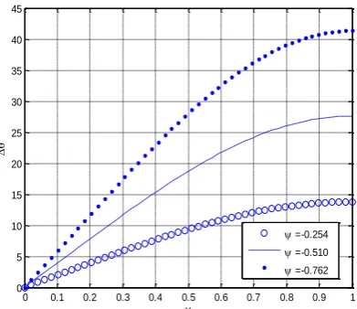
[image:5.595.53.249.150.319.2]

smaller or large gap between the temperature distribution in the case of with and without heat source.

[image:5.595.55.526.360.727.2]

Figure 5. The percentage of the temperature variation “Δθ” for M=1 at various values of ψ

Figure 6 demonstrates the fin efficiency of the wide range of parameter (M) when the heat source parameter ψ = 0. The fin efficient is a maximum near to the wall and decreases rapidly. The fin efficiency far away from the base of the fin becomes almost constant.

Figure 6. The fin efficiency for various values of M with ψ = 0

Conclusion

In this study the numerical solution of the rectangular fin with heat source was verified by the exact solution. The second order non-homogenous differential equation was solved analytically and numerically. The temperature distributions along the fin were plotted for various values of parameter (M) for ψ =0, no heat source and ψ≠0, with heat source. The influence of the heat source on the temperature profiles was investigated as well. The fin efficiency was discussed in the case of the heat source ψ = 0 for the wide range of parameter (M).

Acknowledgement

The author would like to acknowledge the support of Taibah University, KSA.

Nomenclature

Cross-section area of the fin

Convective heat transfer in W/m2-K

Normalized temperature

Fluid temperature in oC

Base temperature in oC

Length of the fin

Height of the fin

Width of the fin

Convective heat transfer in W

Convection/conduction ratio

Heat Flux in W/m2

(6)

Page 6

Fin efficiency

X Spatial dimensionless

x Longitude coordinate

Fin heat transfer in W

Fin surface area in m2

M Convection/Conduction

ratio[dimensionless]

Heat sources parameter

Subscript

b Base

∞ Infinity

c Cross-section

Reference

[1] Shahnor Basri, M. M. Fakir, F. Mustapha, D. L. A. Majid, A. A. Jaafar, Heat Distribution In Rectangular Fins Using Efficient Finite Element And Differential Quadrature Methods, 2009, Engineering, Scientific Research

[2] Antonio Acosta-Iborra and Antonio Campo, Approximate Analytic Analysis Of Annular Fins WithUniform Thickness By Way Of The Mean Value Theorem For Integration That Avoids Modified Bessel Functions, 2013, Latin American and Caribbean Journal of Engineering Education Vol. 7(1). [3] Hyung Suk Kang, Optimization of a Triangular Fin with Variablem Fin Base Thickness, 2007, International Journal of

Mechanical, Aerospace, Industrial and Mechatronics

Engineering Vol:1 No:1.

[4] S. Sunil, J. R. N. Reddy, C. B. Sobhan , Natural convection heat transfer from a thin rectangular fin with a line source at the base Ð a finite difference solution, 1996, Heat and Mass Transfer 31 (1996) 127Ð135 ( Springer-Verlag. [5] Lien-Tsai Yu and Chao-Kuang Chen, Application of Taylor transformation to optimize rectangular with variable thermal parameters, 1998, Applied Mathematical Modeling 22 11±21.

[6]A.A.Walunj,V.S. Daund,andD.D.Palande, Review of Performance of Rectangular Fins under Natural Convection at Different Orientation of Heat Sink,2004 International Journal of Innovation and Applied Studies ISSN 2028-9324 Vol. 6 No.pp. 232-238.

[7]C. Harley and R.J. Moitsheki, Numerical investigation of the temperature profile in a rectangular longitudinal fin, 2013, Nonlinear Analysis: Real World Applications 13 2343–2351. [8] Raseelo J. Moitsheki and Atish Rowjee, Steady Heat Transfer through a Two-Dimensional Rectangular Straight Fin, 2011 Mathematical Problems in Engineering Volume Article ID 826819.

[9] Masoud Asadi and Ramin Haghighi Khoshkho, Temperature Distribution along a Constant Cross Sectional Area Fin,2013, International Journal of Mechanics and

Applications , 3(5): 131-137 DOI:

10.5923/j.mechanics.20130305.04.

[10] A. Moradi, Analytical Solution For Fin With Temperature Dependent Heat Transfer Coefficient,2011, International Journal of Engineering & Applied Sciences (IJEAS) Vol.3, Issue 21-12.

[11] Antonio Campo and Ignacio Lira, Simple approximate analytic treatment of annular fins of variable profile in a heat transfer course, 2012, Latin American and Caribbean Journal of Engineering Education, Vol. 6(1).

Analytical and Numerical Solution of One Dimensional a Rectangular Fin with an Additional Heat Source

Page 1