© 2016, IRJET | Impact Factor value: 4.45 | ISO 9001:2008 Certified Journal | Page 3010
PID Controller for Longitudinal Parameter Control of Automatic
Guided Vehicle
Sheilza Jain
1, Subodhkant
21
Assistant professor, Electronics Engg. Department
YMCA UST, Faridabad- 121006, India
[email protected]
2
M.Tech Student
Electronics Engg.Department
YMCA UST, Faridabad- 121006, India
[email protected]
---***---Abstract -
An automatic guided vehicle (AGV) powered by abattery or an electric motor, is an unmanned, computer controlled mobile transport unit. The development of automatic guided vehicles is one of the areas of research in flexible manufacturing (FMS) to carry out number of task in field of logistic areas. In this paper, open loop characteristics of AGV for longitudinal parameters have been analyzed on the basis of its open loop time and frequency response characteristics. The open loop response of longitudinal model of AGV is not satisfactory, so to improve the response of longitudinal modal of AGV, different types of controller have been used. This paper presents the longitudinal parameter control of AGV by using P, PI, and PID controller. The implementation and simulation of different types of controllers have been done on MATLAB software tool. The comparative analysis of different parameters of AGV has been shown to justify the preference of particular controller.
Key Words: Automatic guided vehicles, longitudinal parameters, modelling and Identification, proportional, PI and PID controller
1. INTRODUCTION
Initially, the AGV is developed as transport device to assist manufacturing system. In the industrial robotics field, these are termed as transport vehicles driven by a computer system. Further, an automatic guided vehicle (AGV) also known as a self-guided vehicle, are programmed to drive to specific points and perform designated functions. These are becoming increasingly popular worldwide in applications which required repetitive actions over a distance. These are largely used to material and load handling applications which includes load transferring, pallet loading/unloading and tugging/towing [1-3]. Different models of AGV such as forked, tug/tow, small chassis and large chassis/unit load, have various load capacities and design characteristics. Its multiplex applications included the aerospace industries,
agriculture industries, metal industries, automotive hospital, paper industries and general any system of transport and storage. According to specific uses and load requirements, AGVs now a days, are available in various sizes and shapes [4].
This paper starts with the mathematical modelling and identification of longitudinal model of AGVs followed by open loop analysis of its longitudinal parameters [5]. In the next section, to improve the response of longitudinal model of AGV, control of AGV has been presented. In this section different types of controllers such as P, PI and PID controllers are tuned to get the desired characteristics of AGVs.
2. IDENTIFICATION AND MODELING OF AGV
Generally, AGVs consist of onboard microprocessors and supervisory control system that helps in various tasks, such as tracking and tracing a modules and generating and/or distributing transport orders to perform a specific task [6-8]. These are able to navigate a guide path network that is flexible and easy to program. Laser, camera, optical, inertial and wire guided systems are used as navigation methods on AGVs. AGVs are programmed for many different and useful maneuvers, like spinning and side-traveling, which allow for more effective production. Some are designed for the use of an operator, but most are capable of operating independently.
© 2016, IRJET | Impact Factor value: 4.45 | ISO 9001:2008 Certified Journal | Page 3011
Figure1Schematics of AGV Robot [10](1)
(2)
(3)
(4)
The kinematic model of AGV includes the physical parameters of robot described by the AGV equations given by equation 1 to 4, wheel parameters and general robot dimensions. The general geometric parameters of AGVs are given in figure 2.
Figure 2 General geometric parameters of the robot. [10]
In kinematical model of AGVs, the wheel variables are described by the equations 5 to 8 where and are the wheel angular velocity.
(5)
(6)
(7)
( 8)
The restrictions of the model are presented by Ollero et al [9]. The dynamical model, respect to the robot coordinate system, is described by equations 9 to 22.
(9)
(10)
m
(11)
(12)
The restrictions of the model are presented by Ollero et al [9]. The dynamical model, respect to the robot coordinate system, is described by equations 9 to22.
m
(13)
In function of wheel variables, is presented the equation system 14:
(14)
The moment equations of robot are described in equations 15 to 21, where I is the inertia tensor of robot.
© 2016, IRJET | Impact Factor value: 4.45 | ISO 9001:2008 Certified Journal | Page 3012
(16)
I
(17)
( 18)
The robot will be symmetric at plane (zr, xr) and (zr, yr) thus the inertia tensor is a diagonal matrix.
(19)
( 20)
With non-slip conditions [11] and movement only at plane (x, y) the equations system is:
(21)
In function of wheel variables and dimensions of robot, is presented the equations system 22
(22)
3. MODEL FOR LONGITUDINAL PARAMETER
CONTROL
An approximated longitudinal model of the vehicle dynamics proposed by Schwarze [11] is given in terms of transfer function of AGV as:
(23)
Where K is the gain of the system and T is the time constant of n-order pole [8].
Other methods, such as those based on measuring the slope on the inflection point of the S shape response, are also possible but difficult of measuring [11]. The Schwarze’s method is applied to those systems with an S-shape step response, as is the present case. On the experimental curve the times at 10%, 30%, 50%, 70% and 90% of the final value must be measured. Then the relationships t10/t90, t10/t70, t10/t50, t10/t30, t30/t50 and t30/t70 are obtained [9]. With
these values the order of the system n can be obtained graphically. Once n is obtained and with another graphic, the value of the time constant T can be obtained. From the step response of the system, the value of the system gain K can be calculated. From the Schwarze’s method, the parameters obtained are as n = 3, K = 1 and T = 2, approximately. Then the transfer function and hence the longitudinal dynamic model of the vehicle is:
(24)
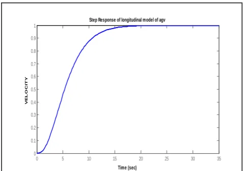
Open loop time and frequency responses of longitudinal modal of AGV are shown in figure 3 and 4 respectively.
0 5 10 15 20 25 30 35
0 0.1 0.2 0.3 0.4 0.5 0.6 0.7 0.8 0.9 1
Step Response of longitudinal model of agv
Time (sec)
V
E
L
O
C
IT
[image:3.595.314.554.267.435.2]Y
Figure 3 Open loop time response of longitudinal modal AGV
-80 -60 -40 -20 0
M
a
g
n
it
u
d
e
(
d
B
)
10-2 10-1 100 101
-270 -180 -90 0
P
h
a
s
e
(
d
e
g
)
Bode Diagram
[image:3.595.326.544.486.676.2]Frequency (rad/sec)
Figure 4 Open loop frequency response of longitudinal modal AGV
© 2016, IRJET | Impact Factor value: 4.45 | ISO 9001:2008 Certified Journal | Page 3013
rise time and to have under dumped system, different typeof controller like P,PI and PID controllers are implemented and simulated.
4. CONTROL SYSTEM DESIGN
[image:4.595.328.544.112.290.2]The control system is designed to manipulate the manipulated variable so that the error between desired output and actual output of the system is minimum or ideally zero [12-13]. Control systems must include some sensing element to sense the output of the system and by making use of feedback and so can, to some extent, adapt to various varying circumstances. The block diagram of simple closed loop system is shown in figure 4.
Fig 4: Block diagram of control system
The error between desired and actual output of the system can be minimized by using different types of controllers such as Proportional P, Proportional Integral PI and Proportional Integral Derivative PID controllers. Depending upon control strategy control action can be taken to minimize the error.
4.1 P Controller
Proportional (P) controller is mostly used in first order processes with single energy storage to stabilize the unstable process. In control system using P controllers, the controller generates the control action directly proportional to the error signal. The main usage of the P controller is to decrease the steady state error of the system. As the proportional gain factor Kp increases, the steady state error of the system decreases. However, despite the reduction, P controller can never manage to reduce the steady state error of the system to zero [4-5, 12]
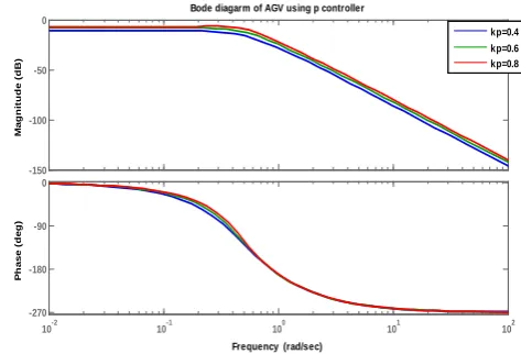
In frequency response, increase in proportional gain, provides smaller amplitude and phase margin, faster dynamics satisfying wider frequency band and larger sensitivity to the noise. This controller can be used only when system is tolerable to a constant steady state error. The step and frequency response of the closed loop system of longitudinal parameters of AGV for different values of controller gain are shown in figures 5 and 6 respectively.
0 5 10 15 20 25 30
0 0.05 0.1 0.15 0.2 0.25 0.3 0.35 0.4 0.45 0.5
Step Response of longitudinal model of AGV with P controller
Time (sec)
A
m
p
li
t
u
d
e
Kp=0.4
[image:4.595.40.284.272.368.2]Kp=0.6 Kp=0.8
Figure 5 Step response of longitudinal model of AGV with P controller
-150 -100 -50 0
M
a
g
n
it
u
d
e
(
d
B
)
10-2 10-1 100 101 102
-270 -180 -90 0
P
h
a
s
e
(
d
e
g
)
Bode diagarm of AGV using p controller
Frequency (rad/sec)
kp=0.4 kp=0.6 kp=0.8
Fig 6 Frequency response of longitudinal model of AGV with p controller
Table: 1 Time response and frequency response characteristics of AGV with different values of P Controller
Parameter Kp=1.5 Kp=2 Kp=2.5
Settling time 14.4 14 13.2
Rise time 5.41 4.66 4.15
Overshoot (%) 3.61% 6.91% 10.4%
Steady state value
0.286 0.375 0.444
Gain margin 19.1db 20.2 21.3
[image:4.595.326.563.334.495.2]© 2016, IRJET | Impact Factor value: 4.45 | ISO 9001:2008 Certified Journal | Page 3014
From the characteristics table 1 as value of proportionalcontroller gain Kp is increasing from 1.5 to 2.5, the settling time and rise time of the closed loop longitudinal model of AGV is decreasing but after further increasing value of the Kp settling time again increasing. Rising time is decreasing. While maximum overshoot of closed loop transfer function and of speed of mobile robot is increasing. From the characteristics table given by table 1, gain margin of the system increases with increase in Kp but phase margin has infinity values at different value of Kp.
As compared to response of open loop longitudinal model AGV, the response of AGV model with P controller reduces the settling time and rise time of AGV system Also the response of the system becomes under dumped as compared to over dumped response of open loop system [5].
It can be easily concluded that use of P controller decreases the rise time, settling time and after a certain value of reduction on the steady state error. Increasing K only leads to overshoot of the system response. P control also causes oscillation if sufficiently aggressive in the presence of lags and/or dead time. The more lags (higher order), the more problem it leads, moreover, it directly amplifies process noise. So, to improve system characteristics, PI controller is used for AGV system.
4.2 PI controller
PI controller is mainly used to eliminate the steady state error resulting from P controller at the cost of speed of the response and overall stability of the system. This controller is mostly used in areas where speed of the system is not an issue [6]. Since PI controller has no ability to predict the future errors of the system, it cannot decrease the rise time and hence the oscillations of the system [12-13]. The transfer function of the PI controller is given as
25
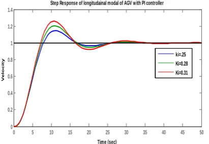
Where KP and Ki are the proportional and integral controllers gain. The time and frequency response of the AGV using PI controller for different values of integral gain are shown in figures 7 and 8 respectively.
0 5 10 15 20 25 30 35 40 45 50
0 0.2 0.4 0.6 0.8 1 1.2 1.4
Step Response of longitudainal modal of AGV with PI controller
Time (sec)
V
e
lo
c
it
y
ki=.25
[image:5.595.327.563.129.293.2]Ki=0.28 Ki=0.31
Fig 7 Step response of longitudinal model of AGV with PI controller
-150 -100 -50 0 50
M
a
g
n
it
u
d
e
(
d
B
)
10-2 10-1 100 101 102
-270 -180 -90 0
P
h
a
s
e
(
d
e
g
)
Bode Diagram of AGV w ith PI controller
Frequency (rad/sec)
[image:5.595.58.264.602.744.2]Ki=.25 Ki=0.28 Ki=0.31
Fig 8 Frequency response of longitudinal model of AGV with PI controller
The analysis of time and frequency response of AGV using PI controller for different values of integral controller’s gain keeping KP constant given by figures 7 and 8 is tabulated in table 2.
Table 2 Time response and frequency response characteristics of AGV with PI controller
At the fixed value of proportional controller gain, Kp=0.9, as increasing in the value of integral gain, Ki=0.25 to 0.35, the settling time and rising time of AGV is increasing but further increasing of gain of integral Ki increases the settling time but decreases the rise time. Further overshoot increases as Ki increases. As shown in table 2, the gain margin of the system increases as Ki increases.
As compared to response of open loop longitudinal model AGV, the closed loop response of AGV system with PI controller has more settling time of system and less rise time than the open loop AGV system. Also, the response of the system becomes under dumped as compared to over dumped of open loop system and hence characteristics of the AGV system improved by using PI controller.
Parameter Ki=1.5 Ki=2 Ki=2.5
Settling time 23.4 24.2 31.08
Rise time 4.44 4.62 4.93
Overshoot(%) 14.8% 20.7 26.2%
Steady state value 1 1 1
Gain margin 8.36db 8.95 9.75
© 2016, IRJET | Impact Factor value: 4.45 | ISO 9001:2008 Certified Journal | Page 3015
4.3 PID Controller
PID controller offers optimum control dynamics such as zero steady state error, fast response, no oscillations and higher stability. The overshoot and the oscillations occurring in the output response of the system decreases by using a derivative gain component in addition to the PI controller. In PID controller, Proportional action responds quickly to changes in error deviation, Integral action removes offsets between the system’s output and the reference and Derivative action speeds up the system response [3, 12-13]. The transfer function KPID of the PID controller is given as
26
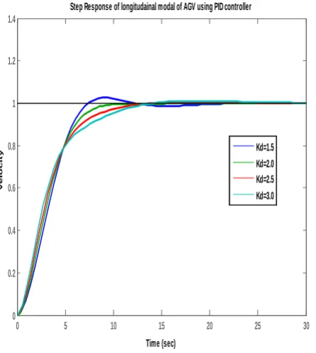
Where KP, Ki and KD are the proportional, integral and derivative controllers gain. The time and frequency response of the AGV using PID controller for different values of derivative controllers gain are shown in figures 9 and 10 respectively.
0 5 10 15 20 25 30
0 0.2 0.4 0.6 0.8 1 1.2 1.4
Step Response of longitudainal modal of AGV using PID controller
Time (sec)
V
e
l
o
c
i
t
y Kd=1.5
Kd=2.0 Kd=2.5
[image:6.595.328.574.115.313.2]Kd=3.0
Fig 9 Step response of longitudinal model of AGV with PID controller
-100 -80 -60 -40 -20 0
M
a
g
n
it
u
d
e
(
d
B
)
10-2 10-1 100 101 102
-180 -135 -90 -45 0
P
h
a
s
e
(
d
e
g
)
Bode Diagram of AGV with PID controller
Frequency (rad/sec)
Kd=1.5
Kd=2.0 Kd=2.5
[image:6.595.63.286.424.673.2]Kd=3.0
Fig 10 Frequency response of longitudinal model of AGV with PID controller
The performance characteristics of AGV using PID controller for different values of derivative controller’s gain are summarized in table 3.
Table 3 Time response and frequency response characteristics of AGV with PID controller
At the fixed value of proportional controller gain, Kp=1.5 and Ki=0.3, the increase in value of derivative controller’s gain Kd=1.5 to 3, the settling time and rising time of the closed loop transfer function of speed of longitudinal model of AGV is decrease but further increasing the value of gain Kd, the settling time increases and rising time again decreases. Moreover, system becomes more damped as Kd increases. From the characteristics table 3, it has been observed that gain margin and phase margin of the system is infinity and -180 respectively for different values of Kd.
Parameter Kd=1.5 Kd=2 Kd=2.5 Kd=3
Settling time 10.1 8.3 10.8 11.8
Rise time 4.66 5.05 5.69 6.72
Overshoot (%)
2.5% 0 0.527% 0
Steady state value
1 1 1 1
Gain margin Infinity Infinity Infinity Infinity
[image:6.595.306.565.436.618.2]© 2016, IRJET | Impact Factor value: 4.45 | ISO 9001:2008 Certified Journal | Page 3016
As compared to response of open loop longitudinal modelAGV, the response of closed loop AGV with PID controller, the settling time and rise time of the AGV system is less than open loop AGV system. Also the response of the system under dumped as compared to over dumped of open loop system which are the desired characteristics achieved by using PID controller.
5. CONCLUSION
As the open loop response of longitudinal model of AGV is not satisfactory, as the required performance characteristics of open loop AGV like settling time and rise time are very large and the system response is over-dumped.
To improve the performance of the longitudinal modal of AGV, the closed loop AGV system with various controllers like P, PI and PID are implemented and simulated.
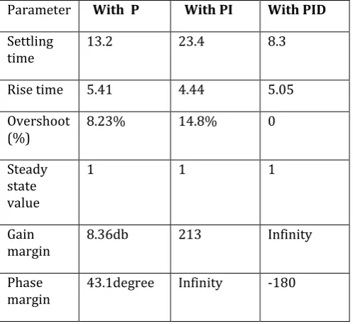
The analysis of table 4 shows that using controllers like P, PI and PID, the response of longitudinal model of AGV has been improved. The time response characteristics like settling time and rise time decreases and the system response becomes under-dumped which are required performance characteristics. In nutshell, the response of closed loop system with controllers like P, PI and PID is fast as compared to the open loop response.
[image:7.595.31.280.422.650.2]
Furthermore, the response of AGV model with PID controller is better than that with the P and PI controller as seen from table 4. PID controller gives less settling time and rise time of the AGV system than those with P and PI controller based AGV system. Hence the performance characteristics of AGV system can be improved by using PID controller.
REFRENCES
[1] J. J. E. Slotine. “The Control Robust of the Manipulators” International journal of Robotics Research, Vol.4, No.2, 1985 [2] Kodagoda, K. R. S., W. S. Wijesoma and E. K. Teoh, “Fuzzy speed and steering control of an AGV” , IEEE Transactions on Control System Technology 10(1), 112—120, 2002. [3] Young Jin Lee, Jin Ho Suh, Jin Woo Lee, and Kwon Soon Lee “Adaptive PID Control of an AGV System using Immune Algorithm and Neural Network Identifier Technique” IEEE International Conference on Control Applications, Taipei, Taiwan, September 2-4,2004
[4] YB. Kim,“ Lateral Control of Autonomous Vehicle using Neural Network Algorithm“. International journal of Automotive Technology, Vo1,.2,pp.71-78, 2002.
[5] Y. 1. Lee. et. al.. “Adaptive Control of Nonlinear System using Immune Response Algorithm”, Proceeding of Asian Control conference, pp.1789-179, 2000
[6] J.Wong. Theory of Ground Vehicles, 2nd ed. Wiley and Sons, New York, 1978
[7] Filed patent certain targets can be even bar-coded and a target counter can sense and counts them as the machine moves along them to keep track of where the vehicle is located as per its desired path, US Patent 4790402 by Field. [8] Suárez, J. I., B. M. Vinagre, A. J. Calderón, C. A. Monje and Y. Q. Chen (2003a).Using Fractional Calculus for Lateral and Longitudinal Control of Autonomous Vehicles. pp. 337-348.Vol. 2809, Lecture Notes in Computer Science. Springer. [9] José Ignacio Suárez, Blas M. Vinagre; Yang Quan Chen, “A Fractional Adaptation Scheme For Lateral Control Of An AGV, IEEE .Control System Magazine 17(3), 23-31.
[10] John Faber Archila and Marcelo becker“Mathematical Modal and design of AGV” IEEE 8th Conference on Industrial Electronics and Applications (ICIE), pp. 1857-1861. [11] 1J. I. Suárez, B. M. Vinagre, F. Gutierrez J. E. Naranjo Y. Q. Chen “Dynamic Models of an AGV Based on Experimental Results” Preprints of the 5th IFAC/EURON Symposium on Intelligent Autonomous Vehicles, Instituto Superior Técnico, Lisboa, Potugal (2004)
[12] Sheilza Aggarwal, Maneesha Garg and Akhilesh “Comparative Analysis of Traditional and Modern Controllers for Piezoelectric Actuated Nano positioner”, International Journal of Nano Devices, Sensors and Systems (IJ-Nano) Volume 1(2), November 2012, pp. 53-64
[13] Nilesh Kumar and Sheilza Jain “Pole Placement Control Technique for Tracking Path Control of UAV by Longitudinal and Lateral Parameters Control”, International Journal on Recent and Innovation Trends in Computing and Communication ISSN: 2321-8169, Volume: 3(10), pp.5815 – 5821.
Parameter With P With PI With PID
Settling
time 13.2 23.4 8.3
Rise time 5.41 4.44 5.05
Overshoot
(%) 8.23% 14.8% 0
Steady state value
1 1 1
Gain
margin 8.36db 213 Infinity
Phase