PARIS RESEARCH LABORATORY
d i g i t a l
June 1991
(Revised, October 1992)
Hassan A¨ıt-Kaci Andreas Podelski
Towards a Meaning of LIFE
Hassan A¨ıt-Kaci Andreas Podelski
A short form of an earlier version of this report was published as [9]. This report is a revision of the earlier report done for publication in the Special Issue on Constraint Logic Programming of the Journal of Logic Programming, edited by Pascal van Hentenryck [10].
The authors can be contacted at the following addresses:
Hassan A¨ıt-Kaci
Digital Equipment Corporation Paris Research Laboratory 85, avenue Victor Hugo 92563 Rueil-Malmaison Cedex France
Andreas Podelski
Laboratoire Informatique Th´eorique et Programmation
2, Place Jussieu 75221 Paris Cedex 05 France
[email protected] [email protected]
c
Digital Equipment Corporation 1991, 1992
LIFE is an experimental programming language proposing to integrate three orthogonal programming paradigms proven useful for symbolic computation. From the programmer’s standpoint, it may be perceived as a language taking after logic programming, functional programming, and object-oriented programming. From a formal perspective, it may be seen as an instance (or rather, a composition of three instances) of a Constraint Logic Programming scheme due to H¨ohfeld and Smolka refining that of Jaffar and Lassez.
We start with an informal overview demonstrating LIFE as a programming language, illustrating how its primitives offer rather unusual, and perhaps (pleasantly) startling, conveniences. The second part is a formal account of LIFE’s object unification seen as constraint-solving over specific domains. We build on work by Smolka and Rounds to develop type-theoretic, logical, and algebraic renditions of a calculus of order-sorted feature approximations.
R ´esum ´e
LIFEy
est un langage de programmation exp´erimental qui propose d’int´egrer trois paradigmes de programmation orthogonaux qui se sont av´er´es utiles pour le calcul symbolique. Du point de vue du programmeur, il peut ˆetre per¸cu comme un langage tenant des styles de programmation logique, fonctionnelle et orient´e-objet. D’une perspective formelle, il peut ˆetre vu comme un exemple (ou plutot, une composition de trois exemples) du sch´ema de programmation par logique de contraintes d ˆu `a H¨ohfeld et Smolka qui raffine celui de Jaffar et Lassez.
Nous commen¸cons par un survol informel d´emontrant LIFE en tant que langage de program-mation, illustrant comment ses primitives offrent des facilit´es peu courantes et peut-ˆetre aussi (plaisamment) surprenantes. La deuxi`eme partie est une description formelle de l’unification d’objets de LIFE vue comme une r´esolution de contraintes dans des domaines sp´ecifiques. Nous appuyons sur des travaux de Smolka et de Rounds pour d´evelopper des pr´esentations tenant de la th´eorie des types, de la logique et de l’alg`ebre, d’un calcul d’approximations de sortes ordonn´ees `a traits.
y
Logic programming, constraint logic programming, functional programming, object-oriented programming, unification, inheritance, feature logic, order-sorted logic, first-order approxima-tion.
Acknowledgements
We acknowledge first and foremost Gert Smolka for his enlightening work on feature logic and for mind-opening discussions. He pointed out that -terms were solved formulae and he also came up, in conjunction with work by Jochen D¨orre and Bill Rounds, with the notion of feature algebras. Bill Rounds has also been a source of great inspiration. In essence, our quest for the meaning of LIFE has put their ideas and ours together. To these friends, we owe a large part of our understanding.
We also wish to express our thanks to Kathleen Milsted and Jean-Christophe Patat for precious help kindly proofreading the penultimate version of the manuscript.
2 LIFE, Informally 2 2.1 -Calculus : : : : : : : : : : : : : : : : : : : : : : : : : : : : : : : : : 3
2.2 Order-sorted logic programming: happy.life : : : : : : : : : : : : 7
2.3 Passive constraints: lefun.life : : : : : : : : : : : : : : : : : : : : 8
2.4 Functional programming with logical variables: quick.life : : : : : 10
2.5 High-school math specifications: prime.life : : : : : : : : : : : : : 11
3 Formal LIFE 12
3.1 The Interpretations: OSF-algebras : : : : : : : : : : : : : : : : : : : : 13
3.2 The syntax : : : : : : : : : : : : : : : : : : : : : : : : : : : : : : : : : 14 3.2.1 OSF-terms : : : : : : : : : : : : : : : : : : : : : : : : : : : : : 14 3.2.2 OSF-clauses : : : : : : : : : : : : : : : : : : : : : : : : : : : : 18 3.2.3 OSF-graphs : : : : : : : : : : : : : : : : : : : : : : : : : : : : : 22
3.3 OSF-orderings and semantic transparency : : : : : : : : : : : : : : : 24
3.4 Definite clauses over OSF-algebras : : : : : : : : : : : : : : : : : : : 29 3.4.1 Definite clauses and queries over OSF-terms : : : : : : : : : : : 29 3.4.2 Definite clauses over OSF constraints : : : : : : : : : : : : : : : 31 3.4.3 OSF-graphs computed by a LIFE program : : : : : : : : : : : : : 32
4 Conclusion 34
A The H ¨ohfeld-Smolka Scheme 35
B Disjunctive OSF Terms 37
... the most succinct and poetic definition: ‘Cr´eer, c’est
unir’ (‘To create is to unify’). This is a principle that must
have been at work from the very beginning of life. KONRADLORENZ, Die R¨uckseite des Spiegels
1 Introduction
As an acronym, ‘LIFE’ means Logic, Inheritance, Functions, and Equations. LIFE also designates an experimental programming language designed after these four precepts for specifying structures and computations. As for what LIFE means as a programming language, it is the purpose of this document to initiate the presentation of a complete formal semantics for LIFE. We shall proceed by characterizing LIFE as a specific instantiation of a Constraint Logic Programming (CLP) scheme with a particular constraint language. In its most primitive form, this constraint language constitutes a logic of record structures that we shall call Order-Sorted Feature logic—or, more concisely, OSF logic.
In this document, we mean to do two things: first, we overview informally the functionality of LIFE and the conveniences that it offers for programming; then, we develop the elementary formal foundations of OSF logic. We shall call this basic OSF logic. Although, in the basic form that we give here, the OSF formalism does not account for all overviewed aspects of LIFE (e.g., functional reduction, constrained sort signature), it constitutes the kernel to be extended when we address those more elaborate issues later elsewhere. Showing how basic OSF logic fits as an argument constraint language of a CLP scheme is therefore a useful and necessary exercise. The CLP scheme that we shall use has been proposed by H¨ohfeld and Smolka [15] and is a generalization of that due to Jaffar and Lassez [16].
We shall define a class of interpretations of approximation structures adequate to represent basic LIFE objects. We call these OSF interpretations. As for syntax, we shall describe three variant (first-order) formalisms: (1) a type-theoretic term language; (2) an algebraic language; and, (3) a logical (clausal) language. All three will admit semantics over OSF interpretations structures. We shall make rigorously explicit the mutual syntactic and semantic equivalence of the three representations. This allows us to shed some light on, and reconcile, three common interpretations of multiple inheritance as, respectively, (1) set inclusion; as (2) algebraic endomorphism; and, (3) as logical implication.
Our approach centers around the notion of an OSF-algebra. This notion was already used implicitly in [1, 2] to give a semantics to -terms. Gert Smolka’s work on Feature Logic [18, 19] made the formalism emerge more explicitly, especially in the form of a “canonicalOSF-graph algebra,” and was used by D¨orre and Rounds in recent work showing undecidability of semiunification of cyclic structures [14].1
1D¨orre and Rounds do not consider order-sorted graphs and focus only on features, whereas Smolka considers
This document is organized as follows. We first give an informal tour of some of LIFE’s unusual programming conveniences. We hope by this to illustrate for the reader that some original functionality is available to a LIFE user. We do this by way of small yet (pleasantly) startling examples. Following that, in Section 3, we proceed with the formal account of basic OSF logic. There, OSF interpretations are introduced together with syntactic forms of terms, clauses, and graphs taking their meaning in those interpretations. It is then made explicit how these various forms are related through mutual syntactic and semantic correspondences. In Section 3.4, we show how to tie basic OSF logic into a CLP scheme. (For the sake of making this work self-contained, we briefly summarize, in Appendix A, the essence of the general Constraint Logic Programming scheme that we use explicitly. It is due to H¨ohfeld and Smolka [15].) Finally, we conclude anticipating on the necessary extensions of basic OSF logic to achieve a full meaning of LIFE.
2 LIFE, Informally
LIFE is a trinity. The function-oriented component of LIFE is directly derived from functional programming languages with higher-order functions as first-class objects, data constructors, and algebraic pattern-matching for parameter-passing. The convenience offered by this style of programming is one in which expressions of any order are first-class objects and computation is determinate. The relation-oriented component of LIFE is essentially one inspired by the Prolog language [13, 17]. Unification of first-order patterns used as the argument-passing operation turns out to be the key of a quite unique and hitherto unusual generative behavior of programs, which can construct missing information as needed to accommodate success. Finally, the most original part of LIFE is the structure-oriented component which consists of a calculus of type structures—the -calculus [1, 2]—and accounts for some of the (multiple) inheritance convenience typically found in so-called object-oriented languages.
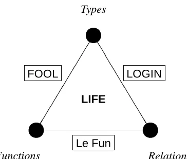
Under these considerations, a natural coming to LIFE has consisted in first studying pairwise combinations of each of these three operational tools. Metaphorically, this means realizing edges of a triangle (see Figure 1) where each vertex is some essential operational rendition of the appropriate calculus. LOGIN is simply Prolog where first-order constructor terms have been replaced by -terms, with type definitions [5]. Its operational semantics is the immediate adaptation of that of Prolog’s SLD resolution. Le Fun [6, 7] is Prolog where unification may reduce functional expressions into constructor form according to functions defined by pattern-oriented functional specifications. Finally, FOOL is simply a pattern-oriented functional language where first-order constructor terms have been replaced by -terms, with type definitions. LIFE is the composition of the three with the additional capability of specifying arbitrary functional and relational constraints on objects being defined. The next subsection gives a very brief and informal account of the calculus of type inheritance used in LIFE ( -calculus). The reader is assumed familiar with functional programming and logic programming.
T T
T T
T T
T T
T T ~
~ ~
Functions Relations
Types
FOOL
Le Fun
LOGIN
[image:11.612.204.386.84.239.2]LIFE
Figure 1: The LIFE molecule
2.1 -Calculus
In this section, we give an informal but informative introduction of the notation, operations, and terminology of the data structures of LIFE. It is necessary to understand the programming examples to follow.
The -calculus consists of a syntax of structured types called -terms together with subtyping and type intersection operations. Intuitively, as expounded in [5], the -calculus is a convenience for representing record-like data structures in logic and functional programming more adequately than first-order terms do, without loss of the well-appreciated instantiation ordering and unification operation.
Let us take an example to illustrate. Let us say that one has in mind to express syntactically a type structure for a person with the property, as expressed for the underlined symbol in Figure 2, that a certain functional diagram commutes.
The syntax of -terms is one simply tailored to express as a term this kind of approximate description. Thus, in the -calculus, the information of Figure 2 is unambiguously encoded into a formula, perspicuously expressed as the -term:
X : person(name)id(first)string; last)S : string);
spouse)person(name)id(last)S); spouse)X)).
person
person
string string
id
id name
-name
-spouse
?
spouse
6
first @ last
@ @
@ R
last
[image:12.612.203.419.73.230.2]
Figure 2: A commutative functional diagram
assume given a set S of sorts or type constructor symbols, a setF of features, or attributes symbols, and a set V of variables (or coreference tags). In the -term above, for example, the symbols person;id;string are drawn fromS, the symbols name;first;last;spouse fromF, and the symbols X;S from V. (We capitalize variables, as in Prolog.)
A -term is either tagged or untagged. A tagged -term is either a variable in V or an expression of the form X : t where X2V is called the term’s root variable and t is an untagged -term. An untagged -term is either atomic or attributed. An atomic -term is a sort symbol inS. An attributed -term is an expression of the form s(`1)t1;. . .;`n)tn)where the root variable’s sort symbol s 2 S and is called the -term’s principal type, the `i’s are mutually distinct attribute symbols inF, and the ti’s are -terms(n0).
Variables capture coreference in a precise sense. They are coreference tags and may be viewed as typed variables where the type expressions are untagged -terms. Hence, as a condition to be well-formed, a -term must have all occurrences of each coreference tag consistently refer to the same structure. For example, the variable X in:
person(id)name(first)string; last)X : string);
father)person(id)name(last)X : string)))
refers consistently to the atomic -term string. To simplify matters and avoid redundancy, we shall obey a simple convention of specifying the sort of a variable at most once and understand that other occurrences are equally referring to the same structure, as in:
person(id)name(first)string; last)X : string);
In fact, since there may be circular references as in X : person(spouse)person(spouse)X)), this convention is necessary. Finally, a variable appearing nowhere typed, as in junk(kind)X) is implicitly typed by a special greatest initial sort symbol>always present inS. This symbol will be left invisible and not written explicitly as in (age)integer;name)string), or written as the symbol@as in@(age)integer;name)string). In the sequel, by -term we shall always mean well-formed -term and call such a form a( )-normal form.
Generalizing first-order terms,2 -terms are ordered up to variable renaming. Given that the setSis partially-ordered (with a greatest element>), its partial ordering is extended to the set of attributed -terms. Informally, a -term t1is subsumed by a -term t2if (1) the principal type of t1is a subtype inSof the principal type of t2; (2) all attributes of t2are also attributes of t1with -terms which subsume their homologues in t1; and, (3) all coreference constraints binding in t2must also be binding in t1.
For example, if student<person and paris<cityname inSthen the -term:
student(id)name(first)string; last)X : string); lives at)Y : address(city)paris); father)person(id)name(last)X);
lives at)Y))
is subsumed by the -term:
person(id)name(last)X : string); lives at)address(city)cityname); father)person(id)name(last)X))).
In fact, if the set S is such that greatest lower bounds (GLB’s) exist for any pair of type symbols, then the subsumption ordering on -term is also such that GLB’s exist. (See Appendix B for the case when GLB’s are not unique.) Such are defined as the unification of two -terms. A detailed unification algorithm for -terms is given in [5].
Consider for example the poset displayed in Figure 3 and the two -terms:
X : student(advisor)faculty(secretary)Y : staff, assistant)X);
roommate)employee(representative )Y))
and:
2In fact, if a first-order term is written f
(t1;. . .;tn), it is nothing other than syntactic sugar for the -term
person
employee
student
staff faculty
workstudy
s1 sm w1 w2 e1 e2 f1 f2 f3
a a
a a
a a
a a
a a
a
@ @
@ @
! ! ! !
J J
J J
A A
A A @
[image:14.612.187.433.73.235.2]@
Figure 3: A lower semi-lattice of sorts
employee(advisor)f1(secretary)employee, assistant)U : person);
roommate)V : student(representative)V); helper)w1(spouse)U)).
Their unification (up to tag renaming) yields the term:
W : workstudy(advisor)f1(secretary)Z : workstudy(representative)Z); assistant)W);
roommate)Z;
helper)w1(spouse)W)).
Last in this brief introduction to the -calculus, we explain type definitions. The concept is analogous to what a global store of constant definitions is in a practical functional programming language based on-calculus. The idea is that types in the signature may be specified to have attributes in addition to being partially-ordered. Inheritance of attributes from all supertypes to a subtype is done in accordance with -term subsumption and unification. For example, given a simple signature for the specification of linear listsS = flist;cons;nilgwith nil<list and cons<list, it is yet possible to specify that cons has an attribute tail ) list. We shall specify this as:
list :=fnil; cons(tail)list)g.
As in this list example, such type definitions may be recursive. Then, -unification modulo such a type specification proceeds by unfolding type symbols according to their definitions. This is done by need as no expansion of symbols need be done in case of (1) failures due to order-theoretic clashes (e.g., cons(tail)list)unified with nil fails; i.e., gives?); (2) symbol subsumption (e.g., cons unified with list gives just cons), and (3) absence of attribute (e.g., cons(tail)cons) unified with cons gives cons(tail)cons)). Thus, attribute inheritance may be done “lazily,” saving much unnecessary expansions [11].
In LIFE, a basic -term denotes a functional application in FOOL’s sense if its root symbol is a defined function. Thus, a functional expression is either a -term or a conjunction of -terms denoted by t1: t2 : . . . : tn.3 An example of such is append(list;L): list, where append is the FOOL function defined as:
list :=f[]; [@jlist]g: append([];L : list)!L:
append([HjT : list];L : list)![Hjappend(T;L)]:
This is how functional dependency constraints are expressed in a -term in LIFE. For example, in LIFE the -term foo(bar)X : list;baz)Y : list;fuz)append(X;Y): list) is one in which the attribute fuz is derived as a list-valued function of the attributes bar and baz. Unifying such -terms proceeds as before modulo suspension of functional expressions whose arguments are not sufficiently refined to be provably subsumed by patterns of function definitions.
As for relational constraints on objects in LIFE, a -term t may be followed by a such-that clause consisting of the logical conjunction of (relational) literals C1;. . .;Cn, possibly containing functional terms. It is written as t jC1;. . .;Cn. Unification of such relationally constrained terms is done modulo proving the conjoined constraints. We will illustrate this very intriguing feature with two examples: prime.life (Section 2.5) andquick.life
(Section 2.4). In effect, this allows specifying daemonic constraints to be attached to objects. Such a (renamed) “daemon-constrained” object’s specified relational and (equational) functional formula is normalized by LIFE, its proof being triggered by unification at the object’s creation time.
We give next some LIFE examples.
2.2 Order-sorted logic programming: happy.life
The first example illustrates a use of partially-ordered sorts in logic programming. The -terms involved here are only atomic -terms; i.e., unattributed sort symbols. This example shows the advantage of summarizing the extent of a relation with predicate’s arguments ranging over types rather than individuals.
3In fact, we propose to see the notation : simply as a dyadic operation resulting in the GLB of its arguments
Peter, Paul and Mary are students, and students are persons.
student := {peter;paul;mary}. student <| person.
Grades are good grades or bad grades. A and B are good grades, while C, D and F are bad grades.
grade := {goodgrade;badgrade}. goodgrade := {a;b}.
badgrade := {c;d;f}.
Goodgrades are good things.
goodgrade <| goodthing.
Every person likes herself. Every person likes every good thing. Peter likes Mary.
likes(X:person,X).
likes(person,goodthing). likes(peter,mary).
Peter got a C, Paul an F and Mary an A.
got(peter,c). got(paul,f). got(mary,a).
A person is happy if s/he got something that s/he likes, or, if s/he likes something that got a good thing.
happy(X:person) :- got(X,Y),likes(X,Y).
happy(X:person) :- likes(X,Y),got(Y,goodthing).
To the query ‘happy(X:student)?’ LIFE answersX = mary (twice—see why?), then givesX = peter, then fails. (It helps to draw the sort hierarchy order diagram.)
2.3 Passive constraints: lefun.life
The next three examples illustrate the interplay of unification and interpretable functions. The first two do not make any specific use of -terms. Again, the first-order term notation is used as implicit syntax for -terms with numerical features.
p(X, Y) :- q(X, Y, Z, Z), r(X, Y). q(X, Y, X+Y, X*Y).
q(X, Y, X+Y, (X*Y)-14). r(3, 5).
r(2, 2). r(4, 6).
Upon a query ‘p(X,Y)?’ the predicate p selects a pair of expressions in X and Y whose evaluations must unify, and then selects values for X and Y. The first solution selected by predicateq sets up the residual equation (or residuation, or suspension) that X + Y= XY (more precisely that both X + Y and XY should unify with Z), which is not satisfied by the first pair of values, but is by the second. The second solution sets up X + Y =(XY) 14 which is satisfied by X=4;Y=6.
The next two examples show the use of higher-order functions such asmap:
map(@, []) -> [].
map(F, [H|T]) -> [F(H)|map(F,T)]. inc_list(N:int, L:list, map(+(N),L)).
To the query ‘inc list(3,[1,2,3,4],L)?’ LIFE answersL = [4,5,6,7].
In passing, note the built-in constant@as the primeval LIFE object (formally written>) which approximates anything in the universe.
Note that it is possible, since LIFE uses -terms as a universal object structure, to pass arguments to functions by keywords and obtain the power of partial application (currying) in all arguments, as opposed to-calculus which requires left-to-right currying [3]. For example of an (argument-selective) currying, consider the (admittedly pathological) LIFE program:
curry(V) :- V = G(2=>1), G = F(X), valid(F), pick(X), p(sq(V)). sq(X) -> X*X.
twice(F,X) -> F(F(X)). valid(twice).
p(1).
id(X) -> X. pick(id).
twice(id,1). Finally, it must be verified that the square of V unifies with a value satisfying propertyp.
2.4 Functional programming with logical variables: quick.life
This is a small LIFE module specifying (and thus, implementing) C.A.R. Hoare’s “Quick Sort” algorithm functionally. This version works on lists which are not terminated with[](nil) but with uninstantiated variables (or partially instantiated to a non-minimal list sort). Therefore, LIFE makes difference-lists bona fide data structures in functional programming.
q_sort(L,order => O) -> undlist(dqsort(L,order => O)). undlist(X\Y) -> X | Y=[].
dqsort([]) -> L\L.
dqsort([H|T],order => O) -> (L1\L2) : where
((Less,More) : split(H,T,([],[]),order => O), (L1\[H|L3]) : dqsort(Less,order => O),
(L3\L2) : dqsort(More,order => O)). where -> @.
split(@,[],P) -> P.
split(X,[H|T],(Less,More),order => O) -> cond(O(H,X),
split(X,T,([H|Less],More),order => O), split(X,T,(Less,[H|More]),order => O)).
The functiondqsorttakes a regular list (and parameterized comparison boolean functionO) into a difference-list form of its sorted version (using Quick Sort). The functionundlist
yields a regular form for a difference-list. Finally, notice the definition and use of the (functional) constantwherewhich returns the most permissive approximation (@). It simply evaluates its arguments (a priori unconstrained in number and sorts) and throws them away. Here, it is applied to three arguments at (implicit) positions (attributes) 1 (a pair of lists),
2 (a difference-list), and 3 (a difference-list). Unification takes care of binding the local variables Less, More, L1, L2, L3, and exporting those needed for the result (L1, L2). The advantage (besides perspicuity and elegance) is performance: replacingwherewith @
inside the definition ofdqsortis correct but keeps around three no-longer needed argument structures at each recursive call.
Here are some specific instantiations:
such that to the query:
L = string_sort(["is","This","sorted","lexicographically"])?
LIFE answers:
L = ["This","is","lexicographically","sorted"].
2.5 High-school math specifications: prime.life
This example illustrates sort definitions using other sorts and constraints on their structure. A prime number is a positive integer whose number of proper factors is exactly one. This can be expressed in LIFE as:
posint := I:int | I>0=true.
prime := P:posint | number_of_factors(P) = one.
where:
number_of_factors(N:posint) -> cond(N<=1,
{},
factors_from(N,2)). factors_from(N:int,P:int)
-> cond(P*P>N, one,
cond(R:(N/P)=:=floor(R), many,
factors_from(N,P+1))). posint_stream -> {1;1+posint_stream}.
list_all_primes :- write(posint_stream:prime), nl, fail.
posint_stream_up_to(N:int) -> cond(N<1,
{},
{1;1+posint_stream_up_to(N-1)}). list_primes_up_to(N:int)
:- write(posint_stream_up_to(N):prime), nl, fail.
This last example concludes our informal overview of some of the most salient features of LIFE. Next, with a slight change of speed, we shall undertake casting its most basic components into an adequate formal frame.
3 Formal LIFE
This section makes up the second part of this paper and sets up formal foundations upon which to build a full semantics of LIFE. The gist of what follows is the construction of a logical constraint language for LIFE type structures with the appropriate semantic structures. In the end of this section, we will use this constraint language to instantiate the H¨ohfeld-Smolka CLP scheme (see Appendix Section A for a summary of the scheme). We hereby give a complete account essentially of that part of LIFE which makes up LOGIN [5] without type definitions. Elsewhere, using the same semantic framework, we account for type definitions [11] and for functions as passive constraints [8].
Thus, the point of this section is to elucidate how the core constraint system of LIFE (namely, -terms with unification) is an instance of CLP. The main difficulty faced here is the absence of element-denoting terms since -terms denote sets of values. It is still possible, however, to compute “answer substitutions,” and we will make explicit their formal meaning. A concrete representation of -terms is given in term of order-sorted feature (OSF) graphs. One main insight is that OSF-graphs make a canonical interpretation. In addition, they enjoy a nice “schizophrenic” property: OSF-graphs denote both elements of the domain of interpretation and sets of values. Indeed, anOSF-graph may be seen as the generator of a principal filter for an approximation ordering (namely, of the set of all graphs it approximates). What we also exhibit is that a most general solution as a variable valuation is immediately extracted from an
Then, all these syntaxes are formally related thanks to explicit correspondences. Following that, Section 3.3 shows that each syntax is endowed with a natural ordering. The terms are ordered by set-inclusion of their denotations; the clauses by implications; and, the graphs by endomorphic approximation. It is then established in a semantic transparency theorem that these orderings are semantically preserved by the syntactic correspondences. The last part, Section 3.4, integrates the previous constructions into a relational language of definite clauses and ties everything together as an explicit instance of the H¨ohfeld-Smolka CLP scheme. Section 3.4.1 deals with definite clauses and queries overOSF-terms; Section 3.4.2 deals with definite clauses ofOSF-constraints; and, Section 3.4.3 deals withOSF-graphs computed by a LIFE program.
3.1 The Interpretations: OSF-algebras
The formulae of basic OSF logic are type formulae which restrict variables to range over sets of objects of the domain of some interpretation. Roughly, such types will be used as approximations of elements of the interpretation domains when we may have only partial information about the element or the domain. In other words, specifying an object to be of such a type does in no way imply that this object can be singled out in every interpretation. Furthermore, it will not be necessary to consider a single fixed interpretation domain, reflecting situations when the domain of discourse can not be specified completely, as is often the case in knowledge representation. Instead, it can be sufficient to specify a class of admissible interpretations. This is done by means of a signature. We shall consider domains which are coherently described by classifying symbols (i.e., partially-ordered sorts) and whose elements may be functionally related with one another through features (i.e., labels or attributes). Thus, our specific signatures will comprise the symbols for sorts and features and regulate their intended interpretation.
An order-sorted feature signature (or simplyOSF-signature) is a tuplehS;;^;Fisuch that:
Sis a set of sorts containing the sorts>and?;
is a decidable partial order onSsuch that?is the least and>is the greatest element; hS;;^iis a lower semi-lattice (s^s
0
is called the greatest common subsort of sorts s and s0
);
F is the set of feature symbols.
A signature as above has the following interpretation. An order-sorted feature algebra (or simplyOSF-algebra) over the signaturehS;;^;Fiis a structure
A=hD A
;(s A
)s 2S
;(` A
) `2F
i
such that:
D A
is a non-empty set, called the domain ofA(or, universe); for each sort symbol s inS, s
A
is a subset of the domain; in particular,> A
=D A
and ?
A =;;
i.e.,(s^s 0 ) A =s A \s 0A
for two sorts s and s0 inS. for each feature`inF,`
A
is a total unary function from the domain into the domain; i.e.,`
A : DA
7!D A
;
Thanks to our interpretation of features as functions on the domain, a natural monoid homomorphism extends this between the free monoidhF
;:;"iand the endofunctions of D A with composition,h(D
A )
(D A
) ;;Id
DAi. We shall refer to elements of either of these monoids as attribute (or feature) compositions.
In the remainder of this paper, we shall implicitly refer to some fixed signaturehS;;^;Fi. The notion of OSF-algebra calls naturally for a corresponding notion of homomorphism preserving structure appropriately. Namely,
Definition 1 (OSF-Homomorphism) An OSF-algebra homomorphism : A 7! B between twoOSF-algebrasAandBis a function: D
A 7!D B such that: (` A
(d))=` B
((d))for all d2D A
;
(s A
) s B
.
It comes as a straightforward consequence that OSF-algebras together with OSF -homomor-phisms form a category. We call this categoryOSF.
Let D be a non-empty set and(`
D
2D
D
) `2Fan
F-indexed family of total endofunctions of D. To any feature composition!=`1:. . .:`n; n0in the free monoidF
, there corresponds a function composition!
D
=`
D n. . .`
D
1 in DD(for n=0;"
D
=1D). Then, for any non-empty subset S of D, we can construct theF-closure of S, the setF
(S)=
S ! 2F
!
D
(S). This is the smallest set containing S which is closed under feature application. Using this, the familiar notion of least algebra generated by a set can naturally be given forOSF-algebras as follows.
Proposition 1 (Least subalgebra generated by a set) Let D be the domain of an OSF -algebraA, then for any non-empty subset S of D, theF-closure of S is the domain ofA[S], the leastOSF-algebra subalgebra ofAcontaining S; i.e., D
A[S] =F
(S).
Proof: F
(S) is closed under feature application by construction. As for sorts, simply take
sA[S] =s
D
\F
(S). It is straightforward to verify that this forms a subalgebra which is the smallest containing S.
3.2 The syntax
3.2.1 OSF-terms
Definition 2 (OSF-Term) An order-sorted feature term (or, OSF-term) is an expression of the form:
=X : s(`1) 1;. . .;`n) n) (1) where X is a variable inV, s is a sort inS,`1;. . .;`nare features inF, n0, and 1;. . .; n areOSF-terms.
Note that the equation above includes n=0as a base case. That is, the simplestOSF-terms are of the form X : s. We call the variable X in the above OSF-term the root of (noted Root( )), and say that X is “sorted” by the sort s and “has attributes”`1;. . .;`n. The set of variables occurring in is given by Var( )=fXg[
S
jnVar ( j).
Example 3.1 The following is an example of the syntax of anOSF-term. X : person(name)N :>(first)F : string);
name)M : id(last)S : string);
spouse)P : person(name)I : id(last)S :>); spouse)X :>)).
Note that, in general, anOSF-term may have redundant attributes (e.g., name above), or the same variable sorted by different sorts (e.g., X and S above).
Intuitively, such an OSF-term as given by Equation 1 is a syntactic expression intended to denote sets of elements in some appropriate domain of interpretation under all possible valuations of its variables in this domain. Now, what is expressed by anOSF-term is that, for a given fixed valuation of the variables in such a domain, the element assigned to the root variable must lie within the set denoted by its sort. In addition, the function that denotes an attribute must take it into the denotation of the corresponding subterm, under the same valuation. The same scheme then applies recursively for the subterms. Clearly, anOSF-algebra forms an adequate structure to capture this precisely as shown next.
Given the interpretationA, the denotation [[ ]] A;
of an OSF-term of the form given by equation 1, under a valuation:V 7!D
A
is given inductively by: [[ ]]A;
=f(X)g \ s A
\ \
1in (`
A
i ) 1
([[ i]] A;
) (2)
where an expression such as f 1(S), when f is a function and S is a set, stands for fxj9y y=f(x)g; i.e., denotes the set of all elements whose images by f are in S.
recovered from the lightened notation, by introducing a new distinct variable anywhere one is missing and introducing the sort>anywhere a sort is missing, denotes precisely the same set, irrespective of the name of single occurrence variables.
Example 3.2 Using this light notation, theOSF-term of Example 3.1 becomes: X : person(name)>(first)string);
name)id(last)S : string);
spouse)person(name)id(last)S); spouse)X)).
Observe that Equation 2 reflects the meaning of an OSF-term for only one valuation and therefore always specifies a singleton or possibly the empty set. Also, note that this definition does include the base case (i.e., n=0), owing to the fact that intersection over the empty set is the universe (T
f. . . j1ing= T
;=D A
).
Since we are interested in all possible valuations of the variables in the domain of an OSF -algebra interpretationA, the denotation of anOSF-term =X : s(`1) 1;. . .;`n ) n)is defined as the set of domain elements:
[[ ]]A =
[
2Val(A) [[ ]]A;
: (3)
The syntax of OSF-term allows some to be in a form where there is apparently ambiguous or even implicitly inconsistent information. For instance, in theOSF-term of Example 3.1, it is unclear what the attribute name could be. Similarly, if string and number are two sorts such that string^number = ?, it is not clear what the ssn attribute is for the OSF-term X :>(ssn)string;ssn)number), and whether indeed such a term’s denotation is empty or not. The following notion is useful to this end.
Definition 3 ( -term) A normalOSF-term is of the form =X : s(`1) 1;. . .;`n) n) where:
there is at most one occurrence of a variable Y in such that Y is the root variable of a non-trivialOSF-term (i.e., different than Y :>);
s is a non-bottom sort inS;
`1;. . .;`nare pairwise distinct features inF, n0, 1;. . .; nare normalOSF-terms.
We call the set that they constitute.
X : person(name)id(first)string; last)S : string);
spouse)person(name)id(last)S); spouse)X))
is a -term and always denotes exactly the same set as the one of Example 3.1.
Given an arbitrary OSF-term , it is natural to ask whether there exists a -term 0 such that [[ ]]A
=[[ 0
]]A
in everyOSF-interpretationA. We shall see in the next subsection that there is a straightforward normalization procedure that allows either to determine whether an
OSF-term denotes the empty set or produce an equivalent -term form for it.
Before we do that, let us make a few general but important observations aboutOSF-terms. First, theOSF-terms generalize first-order terms in many respects. In particular, if we see a first-order term as an expression denoting the set of all terms that it subsumes, then we obtain the special case whereOSF-terms are interpreted as subsets of a free term algebraT(;V), which can be seen naturally as a specialOSF-algebra where the sorts form a flat lattice and the features are (natural number) positions. Recall that the first-order term notation f(t1;. . .;tn) is syntactic sugar for the -term notation f(1)t1;. . .;n)tn):
4
Second, observe that since Equation (3) takes the union over all admissible valuations, it is natural to construe all variables occurring in an OSF-term to be implicitly existentially quantified at the term’s outset. However, this latter notion is not very precise as it is only relative toOSF-terms taken out of external context. Indeed, it is not quite correct to assume so in the particular use made of them in definite relational clauses where variables may be shared among several goals. There, it will be necessary to relativize carefully this quantification to the global scope of such a clause.5 Nevertheless, assuming no further context, theOSF-term semantics given above is one in which all variables are implicitly existential. To convince herself, the reader need only consider the equality [[X : s]]A
= s A
(which follows since S
2Val(A)
(f(X)g \ s A
)= s A
). A corollary of this equality, is that it is natural to view sorts as particular (basic)OSF-terms. Indeed, their interpretations as either entities coincide. Third, another important consequence of this type semantics is that the denotation of an
OSF-term is the empty set in all interpretations if has an occurrence of a variable sorted by the empty sort?.
6 We shall call anyOSF-term of the form X :
?an emptyOSF-term. As observed above, any emptyOSF-term denotes exactly the empty set. Dually, it is also clear that [[ ]]=D
A
in all interpretationsAif and only if all variables in are sorted by>. If is of the form Z :>, we call a trivialOSF-term.
4To render exactly first-order terms, feature positions should be such that i f
(t1;. . .;tn)
=ti is defined only for1in. That is, feature positions should be partial functions. In our case, they are total so that if i>n then
i f(t1;. . .;tn)
=>. Therefore, the terms that we consider here are “loose” first-order terms. 5See Section 3.4 for precise details.
6As a direct consequence of the universal set-theoretic identity: f 1
(A\B)=f 1
(A)\f 1
(B), for any function
Fourth, it is important to bear in mind that we treat features as total functions. There are fine differences addressing the more general case of partial features and such deserves a different treatment. We limit ourselves to total features for the sake of simplicity.7 This is equivalent to saying that, given anOSF-term,
= X : s(`1) 1;. . .;`n) n); and a variable Z2= Var( ), we have:
[[ ]]A;
=[[X : s(`1) 1;. . .;`n ) n;`)Z :>)]] A;
for any feature symbol`2F, anyOSF-interpretationAand valuation2Val(A).
Finally, note that variables occurring in an OSF-term denote essentially an equality among attribute compositions as made clear by, say:
[[X :>(`1)Y :>;`2)Y :>)]] A
=fd2D A
j` A
1(d)=` A 2(d)g:
This justifies semantically why we sometimes refer to variables as coreference tags.
3.2.2 OSF-clauses
An alternative syntactic presentation of the information conveyed byOSF-terms can be given using logical means as anOSF-term can be translated into a constraint formula bearing the same meaning. This is particularly useful for proof-theoretic purposes. A constraint normalization procedure can be devised in the form of semantics preserving simplification rules. A special syntactic form called solved form may be therefore systematically exhibited. This is the key allowing the effective use of types as constraints formulae in a Constraint Logic Programming context.
Definition 4 (OSF-Constraint) An order-sorted feature constraint (OSF-constraint) is an atomic expression of either of the forms:
X : s X
: =Y X:`
: =Y
where X and Y are variables inV, s is a sort inS, and`is a feature inF. An order-sorted feature clause (OSF-clause)1 & . . . &nis a finite, possibly empty conjunction ofOSF-constraints 1;. . .;n(n0).
One may read the three atomic forms ofOSF-constraints as, respectively, “X lies in sort s,” “X is equal to Y,” and “Y is the feature`of X.” The set Var()of (free) variables occurring in an
they are equal modulo the commutativity, associativity and idempotence of conjunction “&.” Therefore, a clause can also be formalized as the set consisting of its conjuncts.
The definition of the interpretation ofOSF-clauses is straightforward. IfAis anOSF-algebra and2Val(A), thenA; j=;the satisfaction of the clausein the interpretationAunder the valuation, is given by:
A;j=X : s iff (X)2s A
; A;j=X
:
=Y iff (X)=(Y); A;j=X:`
:
=Y iff ` A
((X))=(Y); A;j=&
0
iff A;j=andA;j= 0
:
Note that the empty clause is trivially valid everywhere.
We can associate an OSF-term = X : s(`1 ) 1;. . .;`n ) n) with a corresponding
OSF-clause( )as follows:
( )=X : s & X:`1 :
=Y1& . . . & X:`n :
=Yn&( 1)& . . . &( n)
where Y1;. . .;Ynare the roots of 1;. . .; n, respectively. We say that theOSF-clause( )is obtained from “dissolving” theOSF-term .
Example 3.4 Let be the OSF-term of Example 3.1. Its dissolved form ( )is the followingOSF-clause:
X : person & X:name :
=N & N :> & N:first :
=F & F : string & X:name
:
=M & M : id & M:last :
=S & S : string & X:spouse
:
=P & P : person & P:name :
=I & I : id & I :last
:
=S & S :> & P:spouse
:
=X & X :>:
Proposition 2 If theOSF-clause( )is obtained from dissolving theOSF-term , then, for everyOSF-algebra interpretationAand everyA-valuation,
[[ ]]A; =
8 <
:
f(X)g if A;j=( );
; otherwise;
and therefore,
[[ ]]A
=f(X)j2Val(A); A;j=( )g:
We will now define rootedOSF-clauses which, when solved, are in one-one correspondence withOSF-terms.
Given anOSF-clause, we define a binary relation on Var(), noted X
; Y (read, “Y is reachable from X in”), and defined inductively as follows. For all X;Y2Var():
X ; X;
X ; Y if Z
; Y where X:` :
=Z is a constraint in.
A rootedOSF-clauseX is anOSF-clausetogether with a distinguished variable X (called its root) such that every variable Y occurring in is explicitly sorted (possibly as Y : >), and reachable from X. We use
R for the injective (!) assignment of rootedOSF-clauses to
OSF-terms , i.e.,
R
( )=( )
Root( ).
Conversely, it is not always possible to assign a (unique)OSF-term to a (rooted)OSF-clause (e.g., X : s & X : s0
). However, we see next that such a thing is possible in an important subclass of rootedOSF-clauses.
Given anOSF-clauseand a variable X occurring in, we say that a conjunct inconstrains the variable X if it has an occurrence of a variable which is reachable from X. One can thus construct the OSF-clause (X)which is rooted in X and consists of all the conjuncts of constraining X. That is,(X)is the maximal subclause ofrooted in X.
Definition 5 (Solved OSF-Constraints) AnOSF-clauseis called solved if for every vari-able X,contains:
at most one sort constraint of the form X : s, with?<s; at most one feature constraint of the form X:`
:
=Y for each`; and, no equality constraint of the form X
: =Y.
We callthe set of allOSF-clauses in solved form, andR the subset of of rooted solved
OSF-clauses.
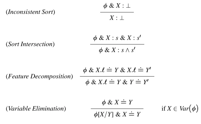
Given anOSF-clause, it can be normalized by choosing non-deterministically and applying any applicable rule among the four transformations rules shown in Figure 4 until none applies. (A rule transforms the numerator into the denominator. The expression[X=Y] stands for the formula obtained fromafter replacing all occurrences of Y by X. We also refer to any clause of the form X :?as thefailclause.)
Theorem 1 (OSF-Clause Normalization) The rules of Figure 4 are solution-preserving, finite terminating, and confluent (modulo variable renaming). Furthermore, they always result in a normal form that is either the inconsistent clause or anOSF-clause in solved form together with a conjunction of equality constraints.
(Inconsistent Sort)
& X :? X :?
(Sort Intersection)
& X : s & X : s 0
& X : s^s 0
(Feature Decomposition)
& X:` :
=Y & X:` : =Y
0
& X:` : =Y & Y
: =Y
0
(Variable Elimination)
& X : =Y
[X=Y] & X : =Y
[image:29.612.126.458.75.280.2]if X2Var()
Figure 4: OSF-Clause Normalization Rules
Termination follows from the fact that each of the three first rules strictly decreases the number of non-equality atoms. The last rule eliminates a variable possibly making new redexes appear. But, the number of variables in a formula being finite, new redexes cannot be formed indefinitely. Confluence is clear as consistent normal forms are syntactically identical modulo the least equivalence onVgenerated by the set of variable equalities.
Givenin normal form, we will refer to its part in solved form as Solved(); i.e.,without its variable equalities.
Example 3.5 The normalization of theOSF-clause given in Example 3.4 leads to the solved
OSF-clause which is the conjunction of the equality constraint N :
= M and the following solvedOSF-clause:
X : person & X:name :
=N & N : id & N:first :
=F & F : string & N:last
:
=S & S : string & X:spouse
:
=P & P : person & P:name :
=I & I : id & I:last
: = S & P:spouse
: = X:
Given a rooted solvedOSF-clauseX, we define theOSF-term (X)by: (X)=X : s(`1) ((Y1));. . .;`n) ((Yn)));
OSF-clauses), and X:`1 :
=Y1;. . .;X:`n :
=Ynare all other constraints inwith an occurrence of the variable X on the left-hand side.
3.2.3 OSF-graphs
We will now introduce the notion of order-sorted feature graph (OSF-graph) which is closely related to those of normalOSF-term and of rooted solvedOSF-clause. The exact syntactic and semantic mutual correspondence between these three notions is to be established precisely.
Definition 6 (OSF-Graph) The elements g of the domain DG
of the order-sorted feature graph algebra G are directed labeled graphs, g = (N;E;N;E;X), where N : N ! S and E: E!Fare (node and edge, resp.) labelings and X2N is a distinguished node called the root, such that:
each node of g is denoted by a variable X, i.e., NV;
each node X of g is labeled by a non-bottom sort s, i.e.,N(N)S f?g; each (directed) edgehX;Yiof g is labeled by a feature, i.e.,E(E)F;
no two edges outgoing from the same node are labeled by the same feature, i.e., if
E hX;Yi
=E hX;Y 0
i
, then Y=Y 0
(g is deterministic);
every node lies on a directed path starting at the root (g is connected).
In the interpretationG, the sort s2Sdenotes the set s G
ofOSF-graphs g whose root is labeled by a sort s0
such that s0
s; that is,
sG
=fg=(N;E;N;E;X)jN(X)sg:
The feature ` 2 F has the following denotation inG. Let g = (N;E;N;E;X). If there exists an edge hX;Yi labeled ` for some node Y of g, then Y is the root of`
G
(g), and the (labeled directed) graph underlying`
G
(g)is the maximally connected subgraph of g rooted at the node Y, g0
=(N jY
;E jY
;N;E;Y). If there is no edge outgoing from the root of g labeled `, then`
G
(g)is the trivial graph of D G
whose only node is the variable Z`;glabeled>, where Z`;g
2V N is a new variable uniquely determined by the feature`and the graph g; that is, if `6=`
0
or g6=g 0
then Z`;g 6=Z
` 0
;g
0. In summary, if g
=(N;E;N;E;X), then:
` G
(g)= 8 < : (N jY ;E jY
;N;E;Y) ifE hX;Yi
=`for somehX;Yi2E; (fZ
`;g
g;;;fhZ `;g
;>ig;;;Z `;g
) where Z`;g 2V N;otherwise.
We will present two concise ways of describingOSF-graphs. The first one assigns to a normal
OSF-term a (unique)OSF-graph G( ). If =X : s, then G( )=(fXg;;;fhX;sig;;;X). If = X : s(`1 ) 1;. . .;`n ) n), and G( i) = (Ni;Ei;N
i;E
i;Xi), then G( ) = (N;E;N;E;X)where:
N=fXg[N1[. . .[Nn;
N(U)= (
s if U=X;
N
i(U) if U2Ni (fXg [ S
i 1 j=1Nj
); E(e)=
(
`i if e=hX;Xii; E
i(e) if e2Ei:
Conversely, we construct a (unique, normal)OSF-term (g)for anyOSF-graph g. If X is the root of g2D
G
, labeled with the sort s2S, and`1;. . .;`nare the (pairwise distinct) features inF, n0, labeling all the edges outgoing from X, then there exists anOSF-term:
(g)=X : s(`1) (g1);. . .;`n) (gn)) where`
G
1(g)=g1, . . . ,` G
n(g)=gn. If, in this recursive construction, the root variable Y of (g
0
)has already occurred earlier in some predetermined ordering ofF
then one has to put Y :>instead of (g
0
). The uniqueness of G( )follows from the fixed choice of an ordering overF
for normalOSF-terms.8
Corollary 1 (Graphical Representation of -Terms) The correspondences : DG !
and G : ! D
G
between normal OSF-terms ( -terms) and OSF-graphs are bijections. Namely,
G = 1
DG and
G = 1 :
Using this one-one correspondence, we can formally characterize theOSF-graph algebra as follows.
D G
=fG( )j is a normalOSF-termg; s
G
=fG(X : s 0
(. . .))js 0
sg; `
G
(G(X : s(. . .;`) 0
;. . .)))= (
G(X : s(. . .;`) 0
;. . .)) if Root( 0
)=X; G(
0
) otherwise;
` G
(G( ))=G(Z `;G( ):
>), otherwise; where Z2= Var( ). Note that, in particular,`
G
(G(X : s(`)X :>))) = G(X : s(`)X :>)). We have defined the following mappings:
: R !
G: DG !
G : !D
G
: ! R somehow “overloading” the notation of mapping (=
+ G
)to work either on rooted solvedOSF-clauses orOSF-graphs.
It follows that Corollary 1 can be extended and reformulated as: 8Without any loss of generality, we may assume an ordering on
Fwhich induces a lexicographical ordering on F
. We require that, in a normalOSF-term of the form above, the features`1;. . .;`nbe ordered, and that the occurrence of a variable Y as root of a non-trivialOSF-term is the least of all occurrences of Y in according to the ordering onF
Proposition 3 (Syntactic Bijections) There is a one-one correspondence between OSF -graphs, normal OSF-terms, and rooted solved OSF-clauses as the syntactic mappings : (R+ D
G
)! , G : !D G
, and: !R put the syntactic domains , D G
, andR in bijection. That is,
1 = GG and G G=1
DG;
1R
=
and
=1 :
Proof: This is clear from the considerations above. The bijection between OSF-graphs and rooted solved OSF-clauses can be defined via OSF-terms. Therefore, we shall take the freedom of cutting the intermediate step in allowing notations such as(g)or G(). It is interesting, however, to see how a solved clausewith the root X corresponds uniquely to an OSF-graph G(X)which is rooted at the node X. A constraint X : s “specifies” the labeling of the node X by the sort s, and a constraint
X:` :
=Y specifies an edgehX;Yilabeled by the feature`. If, for a variable Z, there is no constraint of the form Z : s, then the node Z of G()is labeled>. Conversely, every clause(g)together with the root X of the OSF-graph g is a rooted solved clause, since the reachability of variables corresponds directly to the graph-theoretical reachability of nodes.
As for meaning, we shall presently give three independent semantics, one for each syntactical representation. Each semantics allows an apparently different formalization of a multiple-inheritance ordering. We show then that they all coincide thanks to semantic transparency of the syntactic mappings G, , and.
3.3 OSF-orderings and semantic transparency
Endomorphisms on a givenOSF-algebraAinduce a natural partial ordering.
Definition 7 (Endomorphic Approximation) On each OSF-algebra A a preorder v A is defined by saying that, for two elements d and e in dA
, d approximates e,
dv Ae iff
(d)=e for some endomorphism :A7!A:
We remark that allOSF-graphs are approximated by the trivialOSF-graph G(Z :>)consisting of one node Z labeled >; i.e., for all g 2 D
G
, G(Z : >) v
G g. Clearly an endomorphism : D
G 7! D
G
can be extended from(Z :>)=g by setting(Zi :>)= gi, if` G
i (g)= gi and`
G
i (Z :>)=Zi :>for some “new” variable Zi, etc. . . .
The following results aim at characterizing the solutions of a solved (not necessarily connected) clause in anOSF-algebra. The essential point is to demonstrate that all solutions in anyOSF -algebra of a set ofOSF-constraints can be obtained as homomorphic images from one solution in one particular subalgebra ofOSF-graphs—the canonical graph algebra induced by.
Definition 8 (Canonical Graph Algebra) Let be an OSF-formula in solved-form. The subalgebra G
DG;
of the OSF-graph algebra G generated by D G;
It is interesting to observe that, foranOSF-formula in solved-form, the set D G;
is almost an
OSF-algebra. More precisely, it is closed under feature application up to trivial graphs, in the sense that for all`2F;`
G
(g)2=D G;
)` G
(g)=G(Z `;g:
>). In other words, theF-closure of DG;
adds only mutually distinct trivial graphs with root variables outside Var().
Definition 9 (-Admissible Algebra) Given an OSF-clause in solved form , any OSF -algebraAis said to be-admissible if there exists someA-valuationsuch thatA;j=.
It comes as no surprise that the canonical graph algebra induced by any solvedOSF-clause is-admissible, and so is anyOSF-algebra containing it—G, in particular. The following is a direct consequence of this fact.
Corollary 2 (Canonical Solutions) Every solvedOSF-clause(X)is satisfiable in theOSF -graph algebraGunder anyG-valuationsuch that(X)=G((X)).
In other words, according to the observation made above, the set DG;
contains all the non-trivial graphs solutions. In fact, the canonical graph algebra induced byis weakly initial in OSF(), the full subcategory of-admissible OSF-algebras.
9 This is expressed by the following proposition.
Theorem 2 (Extracting Solutions) The solutions of a solved OSF-clause in any -admissible OSF-algebra A are given by OSF-algebra homomorphisms from the canonical graph algebra induced byin the sense that for each 2Val(A)such thatA;j=there exists anOSF-algebra homomorphism:G
DG;
7!Asuch that:
(X)= G((X))
:
Proof: Let be a solution of inA; i.e., such that A; j= . We define a homomorphism : G
DG;
7! A by setting G((X))
= (X), and extending from there homomorphically. This is possible since the two compatibility conditions are satisfied for any graph g =G((X)). Indeed, if`
G (g)=g
0
, then there are two possibilities: (1) g0
=G(Z :>)where Z2=Var(), or (2)
g0
=G((Y))for some variable Y occurring in; namely, in a constraint of the form X:` :
=Y. Then, `
A
((X))=(Y). This means that for all g2D G;
of the form g=G((X)), it is the case that (`
G (g)=`
A
((g)). If G((X))2s G
(i.e., if G((X))is labeled by a sort s 0
such that s0
s), then contains a constraint of the form X : s
0
, and therefore(X)2s 0A
. This means that if g2s G
then (g)2s
A
and the second condition is also satisfied (if g=G(Z :>), then this is trivially true).
Some known results are easy corollaries of the above proposition. The first one is a result in [19], here slightly generalized from so-called set-descriptions to clauses.
9An object o is weakly initial (resp., final) in a category if there is at least one arrow a : o ! o
0 (resp.,
a : o0
!o) for any other object o 0
For a solved clause , Theorem 2 can be used to infer that the image of a solution in one
OSF-algebra under anOSF-homomorphism (sufficiently defined) is a solution in the other: If 2 Val(A) with A; j= and
0
2 Val(B ) is defined by 0
(X) = ((X)) for some : A 7! B, then simply let
0
: G 7! A be the homomorphism existing according to Theorem 2 (i.e., such that (X) = G((X))
), and then 0
(X) = 0
G((X))
, and thusB ;
0
j= . This fact, a standard property expected from homomorphisms in other formalisms, holds also for a not necessarily solved clause.
Proposition 4 (Extending Solutions) Let A and B be two OSF-interpretations, and let : A 7! B be anOSF-homomorphism between them. Let be any OSF-clause such that A;j=for someA-valuation. Then, for anyB-valuation obtained as =it is also the case thatB ;j=.
Proof: A;j=means thatA;j= 0
for every atomic constraint conjunct 0
of. If 0
is of the form X:`
:
=Y, then` B
(X)
=` B
(X)
= ` A
(X)
= (Y)
=(Y). If 0
is of the form X : s, this means that(X)2s
A
; and then,(X)= (X)
2s B
. Therefore, all atomic constraints inare also true inBunder, and so is.
Theorem 3 (Weak Finality ofG) There exists a totally defined homomorphism from any
OSF-algebraAinto theOSF-graph algebraG.
Proof: For each d 2D A
we choose some variable Xd 2Var to denote a node. There is an edge hXd;Xd
0ilabeled `if`
A (d)=d
0
. Each node Xd is labeled with the greatest common subsort of all
sorts such that d 2s A
(which exists, since we assumeS to be finite). We thus obtain a graph g whose nodes are denoted by variables and labeled by sorts and whose (directed) edges are labeled by features. We define(d)to be the OSF-graph which is the maximally connected subgraph of g rooted in Xdand whose root is Xd. Obviously, we obtain a homomorphism.
In other words, the OSF-graph algebra G is a weakly final object in the category OSF of
OSF-algebras withOSF-homomorphisms. Therefore, we have the interesting situation where, if in the OSF-algebra A a solution 2 Val(A) of an OSF-clause exists, it is given by a homomorphism from theOSF-graph algebraGintoA, and a solution ofinGcan always be obtained as the image ofunder a homomorphism fromAintoG.
Therefore, we may obtain purely semantically as a corollary the following result due to Smolka which establishes that theOSF-algebraGis a “canonical model” forOSF-clause logic [18]:
Corollary 3 (Canonicity ofG) AnOSF-clause is satisfiable iff it is satisfiable in theOSF-graph algebra.
Proof: This is a direct consequence of Theorem 2 and Theorem 3.