402
A NOVEL CHEMICAL REACTION OPTIMIZATION
ALGORITHM FOR HIGHER ORDER NEURAL NETWORK
TRAINING
1K. K. SAHU, 2SIBARAMA PANIGRAHI, 3H. S. BEHERA 123
Veer Surendra Sai University Of Technology (VSSUT), Department Of Computer Science And
Engineering, Burla, 768018, Odisha, India
E-mail: [email protected] , [email protected] , [email protected]
ABSTRACT
In this paper, an application of a novel chemical reaction optimization (CRO) algorithm for training higher order neural networks (HONNs), especially the Pi-Sigma Network (PSN) has been presented. In contrast to basic CRO algorithms, the proposed CRO algorithm used to train HONN possesses two modifications. The reactant size (population size) remains fixed throughout all the iteration, which makes it easier to implement; and adaptive chemical reactions followed by a strictly greedy reversible reaction have been used which assist to reach the global minima in less number of iterations. The performance of proposed algorithm for HONN training is evaluated through a well-known neural network training benchmark i.e. to classify the parity-p problems. The results obtained from the proposed algorithm to train HONN have been compared with results from the following algorithms: basic CRO algorithm and the two most popular variants of differential evolution algorithm (DE/rand/1/bin and DE/best/1/bin). It is observed that the application of the proposed CRO algorithm to HONN training (CRO-HONNT) performs statistically better than that of other algorithms.
Keywords: Artificial Neural Network, Higher Order Neural Network, Pi-Sigma Neural Network, Chemical
Reaction Optimization, Differential Evolution
1. INTRODUCTION
Conventionally artificial neural network (ANN) models have been used predominantly to perform pattern matching, pattern recognition and mathematical function approximation. Compared to traditional ANNs, higher order neural networks (HONNs) have several unique characteristics, including: 1) stronger approximation property; 2) faster convergence; 3) greater storage capacity; and 4) higher fault tolerance capability. Thus, HONN models have shown superior performance than traditional ANNs on forecasting, classification and regression problems.
In this paper the class of HONNs and in particular Pi-Sigma Networks (PSNs) has been studied. The PSNs were introduced by Shin and Ghosh [1]. The PSNs have addressed several difficult tasks such as zeroing polynomials [2] and polynomial factorization [3] more effectively than traditional feed-forward neural networks (FFNNs). Moreover, PSN employ less number of weights than other HONNs, but still manage to incorporate the capability of first order HONN indirectly. The efficiency of HONN models depend on the algorithm used for its training. The objective of any
403 (CRO) is a new optimization technique, inspired by the nature of chemical reactions. CRO has demonstrated excellent performance in solving many engineering problems such as the mining classification rules [14], quadratic assignment problem [11], knapsack problem [15], ANN training problem [16] and multimodal continuous problems. This paper proposes a novel chemical reaction CRO which has better performance than basic CRO algorithm [16] and two most popular variants of DE algorithm, and is used for training the PSN.
The rest of this paper is organized as follows. Section-2 briefly describes the background related to architecture and mathematical model of PSN; chemical reaction optimization; and differential evolution. The proposed training algorithm for PSN has been explained in Section-3. Experimental results are presented in section-4. And finally conclusion and future works are described in Section-5.
2. RELATED WORKS
2.1 PI-SIGMA NEURAL NETWORK (PSN)
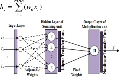
Pi–Sigma Network (PSN) is a feed forward neural network that calculates the product of sum of the input components and passes it to a nonlinear function. The network architecture of PSN (shown in Fig.1) consists of a single hidden layer of summing units and an output layer of product units (instead of summing). The weights connecting the input neurons to the neurons of the hidden layer are adapted during the learning process by the training algorithm, while those connecting the neurons of the hidden layer to the output layer are fixed to one and they are not trainable. Such a network topology with only one layer of trainable weights drastically reduces the training time [1], [17], [18]. Moreover, the product units of PSN gives higher order capabilities which increase its computational power. This is because, the product units enable to expand the input space into higher dimensional space which leads to an easy separation of nonlinearly separable classes where linear separability is possible or a reduction in the dimension of the nonlinearity is achieved. Thus, PSN provides nonlinear decision boundaries offering a better classification capability than the linear neuron (Guler and Sahin, 1994). In addition, Shin and Ghosh (1991) argued that PSNs not only offers better classification over a broad class of problems but also requires less memory and need at least two orders of magnitude less number of computations as compared to MLP for similar performance level.
Consider a PSN with NOIN (number of input neurons), NOHN (number of hidden neurons) and one output neuron. The number of hidden neurons in the hidden layer defines the order of a PSN. For a NOHNth order PSN the number of trainable weights is NOIN × NOHN considering each summing unit is associated with NOIN weights. The output of the PSN is computed by making product of the output of NOHN hidden units and passing it to a nonlinear function, which is defined as follows:
)
(
1
∏
=
=
NOHNj j
h
Y
σ
Where
σ
is a nonlinear transfer function and hj is the output of jth hidden unit which is computed by making sum of the products of each input (xi) with the corresponding weight (wij) between ith input and jth hidden unit. The output of hidden unit is computed as follows:∑
=
=
NOINi
i ij
j
w
x
h
1
[image:2.612.315.520.331.465.2])
(
Figure 1: Architecture of a Typical Pi-Sigma Network
2.2 CHEMICAL REACTION OPTIMIZATION
404 monomolecular reactions assist in intensification while the bimolecular reactions give the effect of diversification. The CRO can be thought of as a new evolutionary technique. The reactants or molecules are similar to chromosomes; the atoms are similar to genes; enthalpy/entropy is equivalent to fitness function; different reactions are similar to crossover and mutation strategies; and reversible reaction is equivalent to selection procedure of any evolutionary algorithm. The major difference between CRO and other evolutionary techniques is that, the population size (that is the number of reactants) may vary from one generation to other where as in evolutionary techniques the population size remains fixed. To have an elaborated description regarding CRO algorithm, interested readers may go through the tutorial of CRO [19]. Every chemical reaction optimization algorithm consists of following steps:
Step 1: Problem and algorithm parameter initialization
Step 2: Setting initial reactants (chromosomes) and evaluation of entropy/enthalpy (fitness function)
Step 3: Applying Chemical reactions (equivalent to mutation and crossover strategies)
Step 4: Reactants update (Equivalent to Selection)
Step 5: Termination criteria check if satisfied go to step-6 otherwise go to step-3
Step 6: Use the reactant having best enthalpy (for minimization)/entropy (for maximization) as the solution.
2.3 DIFFERENTIAL EVOLUTION
The differential evolution (DE) algorithm is a simple and efficient stochastic direct search method for global optimization of multimodal function over a continuous space, was introduced several years ago (1997) [4]. Since then it has been upgraded intensively in recent years [20].Compared to most other EAs, DE is much more simple and straightforward to implement. Although particle swarm optimization (PSO) is also very easy to code, the performance of DE and its variants outperforms the PSO variants over a wide variety of problems as has been indicated by studies like [22], [23] and the CEC competition series. Hence, for comparative performance analysis of the proposed training algorithm, the two most popular variants of DE i.e. DE/best/1/bin and DE/rand/1/bin have been used. The conventions used above is DE/a/b/c, where ‘DE’ stands for ‘differential evolution’, ‘a’ represents the base vector to be perturbed, ‘b’ represents number of difference vectors used for perturbation of ‘a’ and c represents the type of crossover used (bin: binary, exp:
exponential). Interested reader may go through [4], [20] to have a detail description regarding DE algorithm and its variants.
3. CRO-HONNT METHOD
Algorithm 1 (CRO-HONNT)
Set the iteration-counter i=0
/*Randomly Initialize the ReacNum of Reactants from a uniform distribution [U;L]: Pi={R1i, R2i , R3i…., RReacNumi}, with Rji ={ Wj,1i,…….,Wj,Di} for j=1,2,3... ReacNum, D=length of each Reactant (NOIN×NOHN), Wj,k
i
=kth atom of jth reactant in ith iteration representing a weight of PSN.
for j=1 to ReacNum
Calculate the enthalpy e(Rj)
end of for
While (termination criteria is not satisfied) do begin
for j=1 to ReacNum
// perform all reaction over the reactants of Pi Get rand1 randomly in an interval [0, 1]
if rand1 ≤ 0.7
Get rand2 randomly in an interval [0, 1]
if rand2 ≤ 0.5
Decomposition (Rj);
else
Redox1(Rj)
end of if else
Get rand3 randomly in an interval [0, 1] if rand3≤ 0.33
Select the best reactant Rk(Rk≠ Rj) Synthesis (Rj, Rk)
else if rand3≤ 0.66
Select another reactant Rk (Rk≠ Rj) randomly
Displacement(Rj, Rk);
else
Select another reactant Rk(Rk≠ Rj) randomly
Redox2(Rj, Rk)
end of if end of if
Apply strictly greedy Reversible Reaction for increased enthalpy to update reactants
end of for
Set the iteration counter i=i+1
end of while
Use the reactant having best enthalpy as the optimal weight set of PSN.
405 final phase. The initial phase assigns the value to initial parameters like termination criterion, length of reactants/molecules (i.e. number of atoms in a molecule), ReacNum (popsize i.e. total number of reactants in a population) and generates initial reactants. The iteration phase simulates the reaction processes. The reactions may be monomolecular or bimolecular. For monomolecular reaction, Decomposition and Redox1 reactions are considered; and for bimolecular reactions three types of reactions such as: Synthesis, Displacement and Redox2 are considered. The reaction types are chosen considering both intensification and diversification. Moreover, a strictly greedy reversible reaction is used to update the reactants. All the reactions have been elaborated in the following subsequent subsections. In final phase the reactant having best enthalpy is used as the optimal solution (i.e. optimal weight set of a PSN). The pseudo-code of the proposed method is explained in Algorithm 1.
3.1 Reactant Encoding
A set of real numbers are used to represent one reactant, with each reactant corresponding to a weight set of the PSN. The length of a reactant depends on the number of input and hidden neurons of the PSN (i.e. NOIN×NOHN).
3.2 Enthalpy Of A Reactant
Each reactant is associated with some enthalpy. As each reactant represents a weight set of the PSN, the mean square error (MSE) on the train set is considered as enthalpy. The lower the value of enthalpy the better the reactant is. The MSE is defined as follows:
MSE=
NOP
T
Y
NOP
i i i
∑
=1−
2
)
(
Where Yi and Ti are the output of PSN and target for ith train pattern.
3.3 Chemical Reactions
3.3.1 Monomolecular reactions
In monomolecular reactions only one reactant takes part in the reaction and one product is produced by modifying one atom of the reactant. These reactions assist in intensification of the solution by making local search. In our algorithm monomolecular reactions are performed with a probability of 70%, there by glorifying the chances to obtain a better solution around the current solution. Two monomolecular reactions are considered such as: Decomposition and Redox1.
3.3.1.1 Decomposition Reaction
In this reaction a randomly selected atom of the reactant takes part in the reaction. Consider a reactant Rj={Wj,1,Wj,2…….,Wj,D} with Wj,x (x
∈
[1,n]) be an atom of the reactant-j. The pseudo-code of the decomposition reaction is described in Algorithm-2.Algorithm 2 (Decomposition(Rj))
Input: A reactant Rj Duplicate Rj to produce R1
Select an atom x (x
∈
[1, n]) randomly. W1,x=L+ λ × (U-L)Where the rate of reaction (λ) is a random number generated randomly from uniform distribution between [0, 1].
Output: A new reactant R1
3.3.1.2 Redox1 Reaction
It is similar to decomposition reaction except that the rate of reaction(λ)used in this algorithm is obtained randomly from a Cauchy distribution because it diversifies the solution more as compared to traditional normal or uniform distribution. The pseudo-code is described in Algorithm-3.
Algorithm 3 (Redox1(Rj))
Input: A reactant Rj Duplicate Rj to produce R1
Select a point x (x
∈
[1:n]) randomly W1,x =L+ λ × (U-L)Where λ= cauchyrnd(0.5,0.1), is a random number generated randomly from Cauchy distribution with a location parameter 0.5 and scale parameter 0.1. It is regenerated if the random number falls out of the range [0, 1].
Output: A new reactant R1
3.3.2 Bimolecular reactions
Here two reactants Rj={Wj,1,…….,Wj,D} and Rk={Wk,1,Wk,2 …….,Wk,D} will take part in the reaction. These reactions help in diversification of the solution by generating a new solution that is significantly different from the current solution. These reactions occur with a probability of 30%. Below types of bimolecular reactions are used.
3.3.2.1 Synthesis Reaction
406 location parameter ‘M’ and scale parameter 0.1. The value of ‘M’ is initially set to 0.7 and self adaptively determined in the following manner. Mt+1=0.8×Mt+0.2×mean (λsuccess) with t= Number of times the reaction occurs.
Where λsuccess memorizes the successful rate of reactions that generates reactants with better enthalpy than target reactant in the current iteration, thereby glorifying the chance of generating better reaction rates as more and more this reaction occurs. Moreover, the use of best reactant for perturbation intensifies the solutions. Hence, both intensification and diversification can be achieved.
Algorithm 4 (Synthesis (Rj,Rbest))
Input: Two reactants Rj, Rbest R1=RJ+ λ× (Rbest-RJ)
Where
λ
=cauchyrnd(Mt,0.1), is a random number generated randomly from Cauchy distribution with location parameter Mt and scale parameter 0.1. It is regenerated if the random number falls put of the range [0, 1.5].Output: A new reactant R1
3.3.2.2 Displacement Reaction
Two solutions R1 and R2 are obtained from reaction between two reactants Rj and Rk. This reaction is adopted from Bilal altas [14]. The pseudo-code of this reaction is explained in Algorithm 5.
Algorithm 5 (Displacement (Rj, Rk))
Input: Two reactants Rj, Rk R1=λt×Rj+λt × (1- Rk) R2=λt×Rk+λt × (1-Rj)
Where λt is initialized to a random number [0,1]and is updated in the following manner every time this reaction reoccurs (t=number of time the reaction occurs).
λt+1=2.3(λt)2sin(л λt)
Output: Two reactants R1 and R2
3.3.2.3 Redox2 Reaction
Algorithm 6 (Redox2 (Rj,Rk))
Input: Two reactants Rj, Rk R1=Rj+ λ× (Rk- Rj)
Where the rate of reaction (λ) is obtained similar to the way that in synthesis reaction.
Output: A new reactant R1
This reaction is similar to that of synthesis reaction, but here, instead of best reactant a random reactant is selected for the reaction. This reaction assists in more diversification of the solution as compared to synthesis reaction, since in synthesis
reaction the solutions converge towards the best solution.
3.3.3 Reactant update
Every monomolecular or bimolecular reaction is followed by a strictly greedy reversible reaction to update the reactants. In the strictly greedy reversible reaction, for a monomolecular reaction the product produced replaces the reactant that has taken part in the reaction for better enthalpy; and for a bimolecular reaction if two products are produced, these products replace the corresponding reactants for better enthalpy whereas if one product is produced then it replaces the target reactant under consideration. Thus the number of reactants of the population remains same throughout the reaction process. This not only simplifies the algorithm for implementation but also have better performance (in terms of convergence) than the basic CRO algorithm. Moreover, keeping the reactant size fixed avoids the problem of running out of reactants (this may occur if the initial number of reactants is small and number of Redox2 and/or Synthesis reaction is more which produces a product consuming (replacing) two or more reactants taking part in the reaction) in case of variable population size CRO algorithms. The pseudo-code of the strictly greedy reversible reaction is elaborated in algorithm 7.
Algorithm 7 (Reversible Reaction ())
For Monomolecular Reactions
Let Rj under goes monomolecular reaction to produce R1
If enthalpy(R1)<enthalpy(Rj) Replace Rj by R1
end of if
For Bimolecular Reactions
If Rj and Rk under goes reaction to produce R1 (e.g. Synthesis and Redox2 reaction)
If enthalpy (R1) < enthalpy(Rj) Replace Rj by R1
end of if end of if
If Rj and Rk under goes reaction to produce R1 and R2 (e.g. Displacement reaction)
If enthalpy(R1)<enthalpy(Rj) Replace Rj by R1
end of if
If enthalpy(R2)<enthalpy(Rk) Replace Rk by R2
407
4. SIMULATION RESULTS
For comparative performance analysis of proposed training method with DE/rand/1/bin, DE/best/1/bin and CRO [16] to train PSN, parity-p problems (p
∈
[3;6]) have been considered. These problems are widely used benchmarks and are suitable for testing the non-linear mapping and generalization capabilities of training algorithms. The parity-p problem is described as follows: if P represents the number of inputs, and each input can accept values “1” or “−1”, then, the output of the network is “1” if and only if the number of “1” in the inputs of the PSN is odd. Otherwise “−1” occurs in the output of the PSN. Although these problems are easily defined, they are hard to solve, because of their sensitivity to initial weights and possession of large number of local minima. To classify parity-p (p∈
[3;6]) problem, PSNs having structure p-p-1 without bias units were considered and trained using proposed method and other methods for comparison. For each parity problem the training set was equal to the testing set and contained 2p patterns.The termination criterion applied to the training algorithms for parity-p (p
∈
[3;4]) was the mean square training error (MSE) and it was different for each parity problem (0.025,0.0125 respectively); and for parity-p(p∈
[5;6]) was either MSE (0.125, 0.125 respectively, this termination criterion is dominant in the experiments) or maximum generation exceeded (1000, 1000 respectively). These termination criteria have been set based on authors own experience. The PSNs trained here have threshold activation function at output layer; and the upper and lower bound of initial weight sets for parity-p problem is set to 2p to -2p. For DE algorithms the crossover probability Cr and scale factor F were set to 0.7 and 0.5 respectively. For each problem and each algorithm, the popsize (population size/reactant size) is fixed to 10. By making above experimental set up we have conducted 1000 independent simulations using each method for each parity problem. All the simulations were carried out on a system with Intel ® core(TM) 2Duo E7500 CPU, 2.93 GHz with 2GB RAM and implemented using MATLAB (R2009a, The Mathworks, Inc., and Version-7.8.0.347).The following tables show the experimental results for parity-p (p
∈
[3; 6]) problems. The table shows Min the minimum number; Mean the mean value; Max the maximum number; and St.D. the standard deviation of the number of training generations for parity-p (p∈
[3; 6]) problems and the correct classification percentage for parity-p (p∈
[5; 6]). To have a better comparison amongthe methods, we have performed post hoc analysis and ANOVA on the results obtained from 1000 independent simulations for each problem using each method. Correct classification percentage is computed as follows:
Correct classification (%)=
NOP
C
NOP
i i
∑
=1Where NOP is number of testing patterns (NOP=2p); p- Number of inputs to the PSN; Ci- the coefficient representing the correctness of the classification of the ith testing pattern which is determined as follows:
−
=
−
=
=
=
=
Otherwise
0,
1
T
and
1
Y
when
1,
1
T
and
1
Y
when
,
1
C
i ii i
i
Where Yi and Ti are the output of PSN and target for ith test pattern.
TABLE 1:Simulation results on parity-3 problem (best
results in bold)
Algorithms Generations Mean ± St.D. Min Max
CRO-HONNT 1.86 ± 1.64a 1 12
CRO 2.65 ± 4.03c 1 65
DE/rand/1 2.12 ± 1.52b 1 17
DE/best/1 2.11 ± 1.46b 1 9
*Means within a column the same letter(s) are not statistically significant (p=0.05) accordance to Duncan’s Multiple Range Test (SPSS V.16.0.1)
TABLE 2:Simulation results on parity-4 problem (best
results in bold)
Algorithms Mean ± St.D. Min Max Generations
CRO-HONNT 17.41 ± 15.27a 1 187
CRO 23.04 ± 40.49b 1 920
DE/rand/1 18.21 ± 15.38a 1 193
DE/best/1 18.79 ± 15.74a 1 163
*Means within a column the same letter(s) are not statistically significant (p=0.05) accordance to Duncan’s Multiple Range Test (SPSS V.16.0.1)
408 generations taken by proposed algorithm is statistically same to that of DE variants, for parity-3 problem it takes statistically less number of iterations.
TABLE 3:Simulation results on parity-5 problem (best results in bold)
Algorithms Generations Mean ± St.D. Min Max
CRO-HONNT 173.61 ± 160.95a 2 1000
CRO 194.45 ± 235.14b 6 1000
DE/rand/1 245.30 ± 227.84c 10 1000
DE/best/1 248.62 ± 224.79c 5 1000
*Means within a column the same letter(s) are not statistically significant (p=0.05) accordance to Duncan’s Multiple Range Test (SPSS V.16.0.1)
TABLE 4:Simulation results on parity-5 problem (best
results in bold)
Algorithms Correct Classification (%) Mean ± St.D. Min Max
CRO-HONNT 99.87 ± 0.87b 93.75 100
CRO 99.67 ± 1.43a 87.50 100
DE/rand/1 99.82 ± 1.03b 93.75 100
DE/best/1 99.79 ± 1.15b 87.50 100
*Means within a column the same letter(s) are not statistically significant (p=0.05) accordance to Duncan’s Multiple Range Test (SPSS V.16.0.1)
Table-3 and Table-4 show the simulation results obtain on parity-5 problem. It can be observed that, although all methods gave 100% generalization most of the time but none of the methods gave 100% correct classification for all the 1000 independent simulations. The percentage of correct classification by proposed method is not statistical significant to that of DE variants whereas statistically significant to that of traditional CRO methods. However, the proposed method takes statistically less number of generations than other methods to obtain the optimal solutions.
TABLE 5:Simulation results on parity-6 problem (best results in bold)
Algorithms Generations Mean ± St.D. Min Max
CRO-HONNT 783.49 ± 275.93c 28 1000
CRO 728.97 ± 340.57b 23 1000 DE/rand/1 535.43 ± 332.98a 29 1000
DE/best/1 547.46 ± 336.36a 30 1000
*Means within a column the same letter(s) are not statistically significant (p=0.05) accordance to Duncan’s Multiple Range Test (SPSS V.16.0.1)
Table-5 and Table-6 show the experimental results for parity-6 problem. None of the methods gave perfect generalization capabilities for parity- 6 problem for all the 1000 simulations. Although the
proposed method takes significantly more number of generations to attain the termination criteria, but have shown significantly superior performance in terms of classification accuracy than the other methods considered.
TABLE 6:Simulation results on parity-6 problem (best results in bold)
Algorithms Correct Classification (%) Mean ± St.D. Min Max
CRO-HONNT 97.58 ± 3.20c 81.250 100 CRO 94.02 ± 3.69a 78.125 100
DE/rand/1 95.12 ± 5.52b 78.125 100
DE/best/1 95.21 ± 5.30b 78.125 100
*Means within a column the same letter(s) are not statistically significant (p=0.05) accordance to Duncan’s Multiple Range Test (SPSS V.16.0.1)
5. CONCLUSION
In this paper, we have studied HONN models especially; the Pi–Sigma network and used a novel chemical reaction optimization for its training. The use of CRO-HONNT method incorporates efficient and effective searching mechanisms, such that it has less chance to trap to local minima and thus enhance the higher order neural network training procedure. Additionally, this method provides the ability to apply them for training “hardware friendly” PSNs, i.e. PSNs with threshold activation functions and small integer weights can be easily implemented using hardware. The simulation results demonstrate that the proposed training algorithm has superior performance when compared with most popular DE variants and traditional CRO for all test instances considered. The new training algorithm obtains statistically better solutions (e.g. parity-5, 6) and converges quickly (e.g. parity-3, 4, 5) than other evolutionary algorithms considered. Moreover, the fixed population sized CRO makes it easier to implement and still has superior performance than variable sized CRO method.
REFRENCES:
[1] Y. Shin and J. Ghosh, “The pi–sigma network: An efficient higher-order neural network for pattern classification and function approximation”, International Joint
Conference on Neural Networks, 1991.
[2] D. S. Huang, H. H. S. Ip, K. C. K. Law and Z. Chi, “Zeroing polynomials using modified constrained neural network approach”, IEEE Transactions on Neural Networks, Vol. 16, No. 3, 2005, pp. 721–732.
409 networks: Application to stable factorization of 2-d polynomials”, Neural Processing Letter, Vol.7, No. 1, 1998, pp. 5–14.
[4] R. Storn and K.Price, “Differential evolution- A simple and efficient heuristic for global optimization over continuous spaces”, Journal of Global Optimization, Vol. 11, No.4, 1997, pp. 341-359.
[5] D. Goldberg, “Genetic Algorithms in Search”,
Optimization and Machine Learning. Reading,
MA:Addison-Wesley (1989).
[6] J. Kennedy, R. C.Eberhart and Y.Shi,“Swarm intelligence”, San Francisco, CA:Morgan
Kaufmann, 2001.
[7] K. Socha and M. Doringo, “Ant colony optimization for continuous domains”, Europian Journal of Operation Research, Vol. 185, No. 3, 2008, pp. 1155-1173.
[8] D. T. Pham, A. Ghanbarzadeh, E. Koc, S. Otri, S. Rahim and M. Zaidi, “The bees algorithm- A novel tool for complex optimization problems”, in IPROMSOxford, U.K.: Elsevier, 2006.
[9] H.G. Beyer and H.P. Schwefel, “Evolutionary Strategies: A Comprehensive introduction”, Nat. Comput., Vol. 1, No. 1, 2002, pp. 3-52. [10]K. H. Han and J.H. Kim, “Quantum-inspired
evolutionary algorithm for a class of combinatorial optimization”, IEEE
Transactions on Evolutionary Computation,
Vol. 6, 2002, pp. 580–593.
[11]A. Y. S. Lam and V. O. K. Li, “Chemical-Reaction-inspired metaheuristic for optimization”, IEEE Transactionson on
Evolutionary Computation, Vol. 14, No.3,
2010, pp. 381–399.
[12]A.Y.S. Lam, “Real-Coded Chemical Reaction Optimization”, IEEE Transaction on
Evolutionary Computation, Vol. 16, No. 3,
2012, pp. 339-353.
[13]B. Alatas, “ACROA: Artificial Chemical Reaction Optimization Algorithm for global optimization”, Expert Systems with Applications, Vol. 38, 2011, pp. 13170–13180. [14]B. Altas, “A novel chemistry based
metaheuristic optimization method for mining of classification rules”, Expert Systems with Applications, Vol. 39, 2012, pp. 11080-11088. [15]T. K. Truong, K. Li and Y. Xu, “Chemical
reaction optimization with greedy strategy for the 0–1 knapsack problem”, Applied Soft Computing, Vol. 13, 2013, pp. 1774-1880. [16]J.J.Q. Yu, A.Y.S. Lam and V.O.K. Li,
“Evolutionary Artificial Neural Network based on chemical reaction optimization”, in:
IEEE Congress on Evolutionary
Computation (CEC), 2011, pp. 2083–2090.
[17]J. Ghosh and Y. Shin, “Efficient higher-order neural networks for classification and function approximation”, in: International Journal on Neural Systems, Vol. 3, 1992, pp. 323–350. [18]Y. Shin and J. Ghosh, “Realization of Boolean
functions using binary pi-sigma networks”, in: C. H. Dagli, S. R. T. Kumara, Y. C. Shin (Eds.), Intelligent Engineering Systems through Artificial Neural Networks, ASME Press, 1991, pp. 205–210.
[19]A. Y. S. Lam and V. O. K. Li, “Chemical Reaction Optimization: a tutorial”, Memetic Computing Vol. 4, 2012, pp. 3-17.
[20]S. Das and P. N. Suganthanam, “Differential Evolution: A Survey of the state-of-the-Art”, IEEE Transaction on Evolutionary Computation, Vol. 15, No. 1, 2011, pp. 4-31. [21]M. G. Epitropakis, V. P. Plagianakos and M.
N. Vrahatis, “Hardware-friendly Higher-Order Neural Network Training using Distributed Evolutionary Algorithms”, Applied Soft Computing, Vol. 10, 2010, pp. 398-408.
[22]S. Das, A. Abraham, U. K. Chakraborty and A. Konar, “Differential evolution using a neighbourhood based mutation operator”, IEEE
Transaction on Evolutionary Computation,
Vol. 13, No. 3, 2009, pp. 526-553.