Multi Scale Adaptive Connected Component Labeling for Binary Images

2018 3rd International Conference on Information Technology and Industrial Automation (ICITIA 2018) ISBN: 978-1-60595-607-7

Multi-Scale Adaptive Connected Component

Labeling for Binary Images

Yanchao Xing, Zihan Zhang and Rui Li

ABSTRACT

A multi-scale adaptive connected component labeling Algorithm was proposed. The image was first shrunk by levels of down-sampling, and the smallest image was labeled. Then the labeling result was propagated back to the original image level by level. With the design of joint memory structure, this algorithm needs no extra memory. During the backward propagation, double-layer decision tree was used to speed up searching. The backward propagation could be terminated earlier for

application-specific constrains to fulfill application requirements.1

INTRODUCTION

Binary image connected component labeling is a basic operation for computer vision, widely used in object detection, automatic tracking, robot vision, etc. Traditional algorithms include: (1) contour tracing based algorithms[1]; (2) two-run raster scanning[2]; (3) run-based algorithms[3];(4) multiple scanning and label-propagation[4]; (5) multi-branch tree and divide and conquer based algorithms [5]. According to [6], Light Speed Labeling has the fastest speed on RISC machines.

An adaptive connected component labeling algorithm based on hierarchical structure was proposed, which is through labeling result propagation based on analyzing connectivity between different layers.

1

HIERARCHICAL IMAGES ESTABLISHMENT

Establish the Hierarchical Images

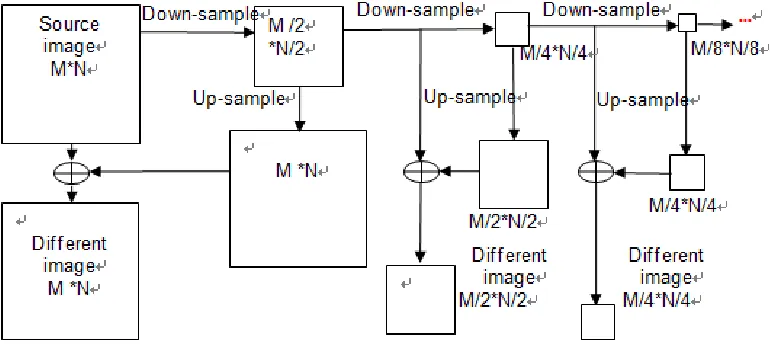
As Figure 1, downs ample images layer by layer, leading to difference pixels between layers, which correspond to edge pixels, or small-sized objects. To record pixel information of a 2*2 block, 4 bits were used, e.g. 1111 means foreground.

Joint Storage of Down-Sampling Results and Label Values for All Layers

To store labeling results, each pixel needs at least one integer, higher bits for pixel patterns, lower bits for labeling results. Smaller size images need no extra storage. As Table I, the image size (width and height) could be reduced to 1/256, where image size could reach 128K * 128K.

Figure 1. The relationship between hierarchical images and difference images.

TABLE I. BIT ALLOCATION FOR JOINT STORAGE OF PIXEL PATTERNS AND LABELING RESULT.

63~40 bits：pixel patterns for all layers 0~39bits：the label of pixels

CONNECTED COMPONENTS LABELING ON SAMLLEST IMAGE

sometime merge equivalence relationship. After the path compression then. (3) finally, performs the label mapping table compression.

BACKWARD PROPAGATION OF THE LABELING RESULTS

Based on upper-layer labeling, check connectivity with neighbors, determine labels for each sub-block with Double Layer Decision Tree. For none labeled neighbors, assign new labels; for same ancestor labels, inherit them; if the connected neighbors have different ancestor labels, merge these ancestor labels.

2 1 3 4

6 9 8 7 0 5 a b c d 8 6 7 9 0 0 add(8) add(7) add(6) add(9) 0 0 1 1 check others check others 1

(a) (b)

Figure 2. (a) Double layer decision tree neighboring relationship. (b) upper-layer decision tree for neighborhoods 6~9.

TABLE II. COMPARISON OF COMPLEXITY OF THREE ALGORITHMS (OPERATION NUMBER PER PIXEL).

Read Write Temporary

assignment

Addition /subtraction

Logical or Bit-wise

Two-pass scanning labeling 3.62 1.54 0.70 4.75 2.70

Light speed labeling 5.62 1.82 3.64 4.85 3.18

Hierarchical labeling (M=4) 4.31 2.01 2.07 6.12 5.48

Hierarchical labeling (M=3) 4.34 2.02 2.07 6.15 5.49

Hierarchical labeling (M=2) 4.46 2.07 2.08 6.30 5.54

Hierarchical labeling (M=1) 4.94 2.26 2.11 6.91 5.82

COMPUTATION COMPLEXITY ANALYSIS

EXPERIMENTS AND RESULT ANALYSIS

There are totally 108 images from USC-SIPI and CIPR. The widths are about 1024, heights from 600 to 700. The platform was ACER Notebook Travel Mate 6292, with Intel Core 2 CPU, T6400 @ 2.00and 2.00 GHz of 2.99 GB memory.

The proportions of difference pixels to foreground pixels for each layer is as shown in Table III and Figure 3. With the increase of the layer index, foreground objects become smaller, so the difference pixel ratio increases, but declines obviously relative to the full image. It's found that images with high difference pixel ratios mainly contain scattered small objects and rich details.

Performance comparisons of hierarchical labeling with different layer number M are shown in Table IV, taking M=1 the base. The speed increases with M, closely related to image content. With the increase of M, the proportion of down-sampling and backward propagation becomes higher, reaching more than 80%.

Table V compares these methods, they have the same order of complexity. The two-pass scanning algorithm with decision tree and path compression has the fastest speed. Decision Tree makes neighborhood connectivity analysis much more efficient, for 95% of the cases, you need to check only the upper pixel label. Path compression makes equivalence merging linear.

The Component-Labeling Algorithm with Contour Tracing can get inner and outer contours, but its performance is greatly affected by the shape and would drop significantly for complex contours image. For light speed labeling algorithm, the variation of processing time is small, so it's much more predictable.

The feature of this algorithm is that it could first find big objects at high layers, whose label values are small (shown in Figure 4). During backward propagation, the constraints mentioned above can be taken into account, to further improve the speed. As the last two columns in Table V, omit the last one or two layers, the processing was significantly faster. If multi-core machine was used, the ideal processing time can be reduced to (0.2 + 0.8 / core number).

Backward propagation without the last few layers has relatively little influence on the subsequent analysis. Table VI shows the percentage of label values (starting from label value one) needed for 95% of the foreground pixels. it's seen that, 80% of the testing images need only the smallest 20% label values, and for 60% of images only the 10% smallest objects.

TABLE III. PROPORTIONS OF DIFFERENCE PIXELS TO FOREGROUND PIXELS ON DIFFERENT LAYERS.

Layer Index 0 1 2 3

proportion of difference pixels 15.8% 23.0% 30.0% 40.2%

Figure 3. Distribution of the proportions of difference pixels to foreground pixels on layer 0~3.

TABLE IV. PERFORMANCE COMPARISON OF HIERARCHICAL LABELING WITH DIFFERENT LAYER NUMBER.

Total process time

Down -sampling

Labeling on the smallest image

Label passing back

Final label write

M=1 1.000 25.7% 18.8% 27.5% 28.0%

M=2 0.932 35.1% 12.3% 38.5% 14.1%

M=3 0.856 43.6% 2.2% 40.4% 13.8%

M=4 0.706 40.1% 1% 42.8% 16.2%

TABLE V. PERFORMANCE COMPARISON OF THE FOUR LABELING ALGORITHMS.

Algorith m

Two pass scanning

Contour Tracing

Light speed labeling

Hierarchica l labeling

Hierarchical labeling without

last layer

Hierarchical labeling without

last two layers

Time 1.000 1.084 1.410 1.578 1.161 1.032

TABLE VI. PERCENTAGE OF LABELS NEEDED FOR DIFFERENT PERCENTAGE OF FOREGROUND PIXELS.

Pixel Percentage 80% 85% 90% 95% 98% 99%

Figure 4. Percentage of labels (from smallest) needed for 95% of the foreground pixels.

CONCLUSIONS

A connected components labeling algorithm based on hierarchical architecture was proposed. It needs no extra space. With DLDT, the connectivity analysis is more efficient. Computation complexity was analyzed. Without increasing processing time and storage space, this algorithm can introduce application-specific constraints into the processing and find big enough objects sooner. This algorithm provides a framework for combining labeling process with application-specific knowledge.

ACKNOWLEGEMENTS

This work was sponsored by Qingdao Source Innovation Program (Special Project for Applied Research - Special Project for Young Scholars) of No. 17-1-1-2-jch.

REFERENCES

1. Chang Fu; Chunjen Chen; Chijen Lu, A Linear-Time Component-Labeling Algorithm Using

Contour Tracing Technique. Computer Vision and Image Understanding, 93(2), 206–220, 2004.

2. Lifeng He; Yuyan Chao; Kenji Suzuki, A New Two-Scan Algorithm for Labeling Connected

Components in Binary Images, Proceedings of the World Congress on Engineering 2012 Vol II, WCE 2012, 445-459, 2012.

3. Lifeng He; Yuyan Chao; Kenji Suzuki, A Run-Based Two-Scan Labeling Algorithm, IEEE

Transactions on Image Processing, Vol. 17, No. 5, 749-756, 2008.

4. Lionel Lacassagne; Bertrand Zavidovique, Light Speed Labeling: Efficient Connected

Component Labeling on RISC Architectures, Journal of Real-Time Image Processing, 6(2), 117-135, 2011.

5. H.L. Zhao; Y.B. Fan; T.X. Zhang; H.S. Sang, Stripe-Based Connected Components Labeling,

Electronics Letters, 46(21), 2010.

6. Cabaret, L.; Lacassagne, L., What is the World's Fastest Connected Component Labeling