Data mining algorithm for manufacturing process control

DOI 10.1007/s00170-004-2367-1 O R I G I N A L A R T I C L E

Hovhannes Sadoyan · Armen Zakarian · Pravansu Mohanty

Data mining algorithm for manufacturing process control

Received: 14 May 2004 / Accepted: 9 August 2004 / Published online: 13 April 2005 ©Springer-Verlag London Limited 2005

Abstract In this paper, a new data mining algorithm based on the rough sets theory is presented for manufacturing process con-trol. The algorithm extracts useful knowledge from large data sets obtained from manufacturing processes and represents this know-ledge using “if/then” decision rules. Application of the data min-ing algorithm developed in this paper is illustrated with an indus-trial example of rapid tool making (RTM). RTM is a technology that adopts rapid prototyping (RP) techniques, such as spray form-ing, and applies them to tool and die making. A detailed discus-sion on how to control the output of the manufacturing process using the results obtained from the data mining algorithm is also presented. Compared to other data mining methods, such decision trees and neural networks, the advantage of the proposed approach is its accuracy, computational efficiency, and ease of use.

Keywords Data mining·Decision rules· Manufacturing process control·Rough sets

Nomenclature

A={a1,a2, . . .,an} Condition attributes set

B={b1,b2, . . .,bm}Decision attributes set

equivalence class set of objects that have the same values for attributes in set A or B

Ai Equivalence classes of A, where i=1, . . .,p

Bj Equivalence classes of B, where j=1, . . .,q

V(Ai,ak) Values of the attributes in equivalence classes

of Ai

H. Sadoyan (u) · A. Zakarian

Department of Industrial and Manufacturing Systems Engineering, USA

E-mail: {shovhans,zakarian}@umich.edu Tel.: +1-313-593-5244

Fax: +1-313-593-3692 P. Mohanty

Department of Mechanical Engineering, University of Michigan – Dearborn, Dearborn, MI 48128, U.S.A. E-mail: [email protected] Tel.: +1-313-593-5244 Fax: +1-313-593-3692

V(Bj,bl) Values of the attributes in equivalence classes

of Bj

Xij Intersection of Aiand Bj

P Percent of objects in a current equivalence class of condition attribute set that corres-pond to a rule; measures rule confidence Q Percent of objects in current equivalence

class of decision attribute set that correspond to a rule

C Percent of objects that correspond to a rule; measures rule support

QTY Quantity of objects corresponding to a rule.

1 Introduction

Data mining is a new area of computational intelligence that offers new theories, techniques and tools for processing and ana-lyzing large datasets. It is a discipline of growing interest and importance. Its application area can provide significant compet-itive advantages to a manufacturing organization by exploiting the potential of large data warehouses.

Currently, one of the most widely used approaches in data mining are decision trees generated through symbolic inductive algorithms [1–4]. Each branch node in a decision tree represents a choice between a number of alternatives, and each leaf nodes represents a classification or decision. When a new object is clas-sified, the values of the object attributes are propagated through the nodes of the tree to the leaf (decision). Decision trees, such as the ID3 or C4.5 designs described in [4–6], use the maximum generality bias to achieve a high predictive accuracy. Kusiak [7] provides a brief description of several decision trees based algo-rithms. The disadvantage of this method is that it uses probability estimates to evaluate the quality of inductive rules. Unreliable probability estimates resulting from a small number of training instances often produces high error rates and occasionally identi-fies patterns that are of no value to the system analyst. Also, de-cision tree induction algorithms require large computer memory to analyze and fit the training dataset. This limits the application of decision tree algorithms to small size problems [8–10].

Neural networks are an alternative technique for pattern recognition in complex and large datasets [11–13]. They are data-driven, self-adaptive methods that use universal functional approximations to estimate any function with arbitrary accu-racy. Neural network-based approaches have been widely used to solve data mining problems in manufacturing, design, and medicine. Zhang [13] provides a detailed survey of neural network algorithms for classification. Riplay and Riplay [14] present a review of the application of several neural network techniques in medicine, including methods for diagnosis and prognoses tasks and survival analysis. Most applications of neural networks in medicine refer to classification tasks. A com-prehensive list of medical neural network applications can also be found in Baxt [15]. One of the main disadvantages of neural network is that it requires large computational time to analyze data compared to other data mining techniques, such as decision trees or rough sets (RS) theory (described in the paper).

Ostermark [16] presented the multi-group classification algo-rithm based on a hybrid fuzzy neural network. A key feature of the approach is the adaptation of the membership function to a new data. They have tested the algorithm with real economic data and results have suggested economically-meaningful interpretations.

Hemsathapat et al. [17] show an application of neuro-fuzzy-genetic data mining architecture in an American charitable or-ganization’s donor database. They combined the application of several techniques to obtain successful results. In their data min-ing approach, after usmin-ing a preprocessmin-ing function as the first step, principal component analysis (PCA) is used to reduce the variables that describe the major trends in the data. Once the ma-jor trends are identified, a probabilistic neural network is used to classify the dataset according to the groups considered. A rule extraction technique and genetic algorithms were used to extract hidden knowledge and to eliminate weak rules, respectively.

The major drawback of decision trees and neural networks is that they are computationally complex, make decisions essential for all objects with unknown outcomes with some error, and re-quire specialized software and hardware. In this paper, new data mining and knowledge extraction algorithms based on RS

the-ory are presented that allow one to analyze and identify useful patterns in datasets.

RS theory, first proposed by Pawlak [18], provides tools for data analysis and autonomous decision-making, and has been used to extract knowledge from datasets. The theory has a strong mathematical foundation and is well suited to deal effectively with various decision problems. Although it overlaps to some extent with fuzzy set theory, RS theory can be viewed as an in-dependent discipline [19]. The primary goal of RS theory is in the classificatory analysis of data [18–20]. For the given dataset, RS algorithms induce a set of relevant concepts which provide data classification. The main advantage of RS theory is that it does not need any preliminary or additional information about the dataset, such as probability in statistics, grade membership or value of possibility in fuzzy set theory. The literature provides several applications of RS theory (see [21–25]).

Kusiak and Kurasek [21] applied a RS-based data mining algorithm to solve a quality-engineering problem in electronics assembly. Using a data mining algorithm, they were able to iden-tify the cause of solder defects in a circuit board. Kusiak [22] presented a new data mining algorithm (G-algorithm) for the knowledge extraction in the form of “if/then” decision rules. G-algorithm was applied to the dataset obtained for children born with a malformation of the heart (tachycardia). The analysis of results shows that the occurrence of tachycardia may be accu-rately predicted for 78.08% of infants using the G-algorithm. Ohrn et al. [23] developed an approach for generating rule-based classifiers based on rough set theory and Boolean reasoning. The approach was applied to a real-world medical dataset. The re-sults showed that with a relatively small number of rules the model was able to accurately describe the patterns in the ori-ginal dataset. Kusiak [24] presented a RS-based approach that combines different decision modes to allow for autonomous decision-making. The approach has been tested on a medical dataset for patients with lung abnormalities. Two independent algorithms were developed to obtain an accurate diagnose. Das-Gupta [25] presented a RS-theory-based data mining approach for the design of information retrieval systems to improve docu-ment indexing. The approach uses Boolean logic, term weight-ing, and approximation space and search strategies to effectively rank the retrieved documents.

In this paper, a new algorithm based on RS theory for manufacturing process control is presented. An application of the algorithm is presented with the industrial example of rapid tool making. The rest of the manuscript is organized as fol-lows: Sect. 2 describes the problem and the mathematical ap-proach; Sect. 3 presents an industrial application of the data mining algorithm and provides a detailed discussion of how to control the output of the manufacturing process using the results obtained from the algorithm.

2 Problem description and mathematical approach

Fig. 1. Phases of the data mining process

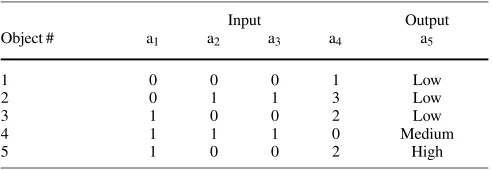
is recognizable to human, for instance using “if/then” decision rules. Figure 1 shows the main steps of a typical data min-ing process. To illustrate these major steps and the data minmin-ing algorithm developed in this paper, consider the sample manufac-turing process dataset in Table 1. Each row (object) in Table 1 represents a single instance (i.e. a single test or experiment) in a manufacturing process. Attributes a1 to a5 denote input and

output parameters of the process.

2.1 Data acquisition

The first step in any data mining approach is the selection of a historical dataset for analysis. A dataset may be retrieved from a single source or may be obtained from several operational databases. Once a dataset is retrieved and organized, data prepro-cessing techniques (as described in the next section) are used to prepare data for analysis.

2.2 Data preprocessing

Data preprocessing is significant in any data mining approach as it may affect the data mining algorithm’s efficiency and accuracy. Data preprocessing, as presented in this paper, consists of data cleaning, data clustering, and attribute reduction.

2.2.1 Data cleaning

Data cleaning is an optional step in data preprocessing and is used to remove outlying records and objects (rows) with missing, null, or inconsistent values from the dataset. Also, in this step data stored as strings (i.e. attributes with the continuous values) are converted to numerical values.

2.2.2 Attribute reduction

Attribute reduction is used to identify and remove redundant at-tributes from the dataset. It optimizes the knowledge extraction process by reducing the size of the set and helps the user to see dependencies between the attributes. The attribute reduction method presented in this paper uses RS technique to evaluate

Table 1. Sample dataset

Input Output

Object # a1 a2 a3 a4 a5

1 0 0 0 1 Low

2 0 1 1 3 Low

3 1 0 0 2 Low

4 1 1 1 0 Medium

5 1 0 0 2 High

dependency levels between all pairs of attributes and removes the attributes that have a higher level of dependency compared to the user’s established threshold. The assumption here is that if the dependency level between two attributes is greater than some user established threshold, then either the first or the sec-ond attribute may be removed from the dataset without the loss of useful information. The dependency level K of attribute aj

from attribute aiis determined from the following:

K(ai,aj)=

L∈a∗_j ai(L)

N (1)

ai(L)= ∪

Y∈a∗_iY⊆L (2)

where:

a∗_i,a∗_j is the equivalence class of attributes aiand aj, respectively.

The equivalence class is the set of objects that have the same value for attribute aiand aj).

L is the equivalence class of ajused in Eq. 1

Y is the equivalence class of aiused in Eq. 2

N is the total number of objects in the dataset

|•| is the cardinality of a set (i.e. number of elements in the set)

ai(L) is the lower approximation of set L over attribute ai (i.e.

the union of equivalence classes of ai which are

com-pletely included in the given set L)

When the dependency level K(ai,aj)=0, then the attribute aj

is independent from the attribute ai. When K(ai,aj)=100 then

aiis fully dependent on aj. This means that for each unique value

of attribute aj there is a corresponding unique value of attribute

ai(i.e. each equivalence class of aiis fully included in one of the

equivalence classes of aj). It is important to emphasize that the

at-tribute ajcannot be removed from dataset based only on the value

of K(ai,aj). The dependency K(aj,ai)should also satisfy the user

established threshold requirements for one of the attributes aior

ajto be removed. In other words, for either attribute aior ajto be

removed from the dataset min{K(ai,aj),K(aj,ai)}must exceed

Table 2. Summary of dependency levels calculations

Attribute Input Output

Attribute a1 a2 a3 a4 a5

a1 – 0 0 100 40

a2 0 – 100 100 40

a3 0 100 – 100 40

a4 0 0 0 – 40

a5 40 0 0 60 –

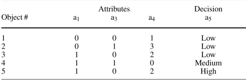
Table 3. Reduced dataset

Attributes Decision

Object # a1 a3 a4 a5

1 0 0 1 Low

2 0 1 3 Low

3 1 0 2 Low

4 1 1 0 Medium

5 1 0 2 High

are strongly connected, a threshold value between 90 and 100% is appropriate; otherwise, it is reasonable to select a threshold be-tween 80 and 90%. To illustrate the attribute reduction method, consider the dataset presented in Table 1 and assume for this ex-ample the user established threshold for the attribute dependency level is 85%. The dependency levels for all the pairs of attributes shown in Table 1 are summarized in Table 2.

One may see from Table 2 that K(a2,a3)=K(a3,a2)=100

(i.e., attributes a2 and a3 are fully dependant), and one of the

attributes a2or a3may be removed from the dataset. The

remain-ing attribute pairs do not satisfy the user threshold requirements and cannot be removed. The datasets which are obtained after the attribute reduction process are shown in Table 3.

2.2.3 Data clustering

Once the data cleaning and attribute reduction steps are com-plete, data clustering algorithms are used (the k-mean [26] or centroid method [27], for example) to discretize attributes with continuous numeric values. This groups continuous numeric values of attributes into numeric ranges (classes). This step helps the data mining algorithm to produce well summarized results and to work more efficiently.

2.3 Decision rules generation

Once the data preprocessing step is complete, a decision rule generation algorithm is used to extract useful knowledge from the dataset. To illustrate the knowledge representation algorithm, the following notation is introduced.

Rule 1: IF a1=0 THEN a5is Low. (P=100%, Q=66.67%, C=40%, QTY=2)

Rule 2: IF a1=1 THEN a5is Medium. (P=33.33%, Q=100%, C=20%, QTY=1)

Rule 3: IF a1=1 THEN a5is High. (P=33.33%, Q=100%, C=20%, QTY=1)

Rule 4: IF a1=1 THEN a5is Low. (P=33.33%, Q=33.33%, C=20%, QTY=1)

Fig. 2. Decision rules generate from the sample dataset

Decision rules generation algorithm

Step 1. Initialize: A= {a1,a2, . . .,an}; B= {b1,b2, . . .,bm}

Step 2. Determine Xij =Ai∩Bj for each i=1, . . .,p and j=

1, . . .,q

Step 3. For each Xij= ∅, generate a rule

IF a1=V(Ai,a1)AND. . .AND an=V(Ai,an)

THEN b1=V(Bj,b1)AND. . .AND bm=V(Bj,bm)

[P, Q, C, QTY]

where: P= |Xij|/|Ai|; Q= |Xij|/|Bj|; C= |Xij|/N;

QTY= |Xij|

In the decision rule generation algorithm, each non-empty in-tersection of the equivalence classes of A and B attribute sets obtained in Step 2 is represented with a single “if/then” decision rule. In this decision rule, the “if” portion of the rule includes the set of attributes representing process conditions (inputs), and the “then” portion of the rule includes the set of attributes that repre-sents process decisions (outputs). The sum (P+Q+C) indicates the importance of the rule and that parameters P, Q, and C in-dividually or jointly provide more insight on rule importance or weakness.

To illustrate the steps of the decision rules extraction al-gorithm and how parameters P, Q, and C are used to analyze the rule, consider the sample dataset provided in Table 3. Here, assume that one wants to obtain “if/then” decision rules to represent the relationships between attributes a1 and a5 of the manufacturing process. In Step 1 of the algorithm, sets A= {a1} and B= {a5} are initialized. In Step 2, the equivalence classes of A and B are determined and their corresponding intersections are calculated as follows:

A1= {1,2},A2= {3,4,5},B1= {1,2,3},B2= {4},B3= {5}. X11=A1∩B1= {1,2},X12=A1∩B2= ∅,

X13=A1∩B3= ∅,X21=A2∩B1= {3},

X22=A2∩B2= {4},X23=A2∩B3= {5}.

In this step the values of the equivalence classes are also determined:

V(A1,a)=0,V(A2,b)=1,V(B1,d)=Low,

V(B2,d)=Medium, and V(B3,d)=High.

In the final step of the algorithm the decision rules are gen-erated and the values of parameters P, Q, C, and QTY are calcu-lated for each rule (see Fig. 2).

P=100% in this rule indicates that all the objects in the dataset that have condition a1=0 are covered by this rule. The value

of Q=100% in Rules 2 and 3 indicate that the objects with the decision outcome a5=Medium and a5=High are covered by

Rules 2 and 3, respectively. One may also see that the lower value of P=33.3%, indicates that condition a1=1 produces

different decision outcomes in the manufacturing process, i.e. a5=Medium, a5=High, and a5=Low in rules 2, 3, and 4,

re-spectively. More detailed discussion on how parameters P, Q, and C are used to analyze the strength and the weakness of the rule is presented in Sect. 3 with an industrial example.

3 Industrial application: rapid tool making

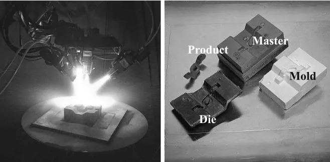
Rapid tool making (RTM), a technology that adopts rapid proto-typing (RP) techniques and applies them to tool and die making, is becoming an increasingly attractive alternative to traditional machining [28]. Among the existing RTM technologies, spray tooling is an emerging and cost-effective technology for a wide variety of manufacturing applications. In the spray tooling pro-cess, tool fabrication begins with a model design represented as a CAD file, which is produced to a master by a RP technology such as fused deposition system (see Fig. 3). A castable ceramic mold is made from this master. Molten metal is sprayed against the ceramic mold, faithfully reproducing the mold shape, details, and texture.

The turnaround is very fast and so far, it has worked well for small stamping tool sets. When the spray-formed tooling pro-cess is scaled-up to manufacture tool sets for stamping doors, hoods and other large body panels, it will save millions of dollars and cut several months off the production process. Therefore, much of the focus at this point is on the development of a pro-cess which can maximize the density of the deposited material, minimize the loss of alloying elements while spraying in the air, and enhance the strength of the tool. In a nutshell, the pro-cess parameters that influence spray propro-cess are: current and the voltage supplied to the spray gun, carrier gas type (argon, ni-trogen or air), gas flow rate, wire type (solid, cored, Boron or Ni/Alum), and the cap type used at the gun tip. The goal of the

Fig. 3. Spray tooling scheme

Fig. 4. The data acquisition process

data mining algorithm when applied to the spray tooling process is to identify the process input parameters that can be used to ef-fectively control spray material characteristics (i.e. the average particle temperature, average velocity, and particle number and size). For example, experiments indicate that to achieve max-imum density and low porosity in the deposited steel, the average particle temperature and velocity at the gun tip should be above 2700 K and 200 m/s, respectively. Therefore, in this study the goal of data mining algorithms is to identify the input param-eters of the spray process that can achieve the target levels of average particle temperature and velocity. The software program developed in C# is used to execute data preprocessing and the rule generation algorithms presented in this paper. An Oracle9i database is used to store and to represent the manufacturing pro-cess data.

3.1 Data acquisition from the spray system

A thermal imaging system (TIS, Stratonics, Inc., Laguna Hills, CA) (see Fig. 4) is utilized to measure the spray process output parameters. For this industrial application, a process dataset con-sisting of 1200 records is used. A representative dataset obtained from the imaging system is shown in Table 4. All the possible values of the input and output process parameters of the process are shown in Table 5.

Table 4. Representative dataset of the spray process

Object Input parameters Output parameters

No Current (A) Voltage (V) Flow rate (cfm) Gas type Wire type Cap dia. (in.) Temp. (K) Velocity (m/s) No. particles

1 200 32 50 N2 Solid 0.250 2741 199.7 530

2 100 36 50 N2 Solid 0.250 2731 197.3 264

3 300 28 50 N2 Solid 0.250 2693 191.5 533

4 200 32 40 N2 Solid 0.250 2917 166.2 24

5 200 32 65 N2 Solid 0.250 2716 240.3 71

6 200 32 50 N2 Cored 0.375 2656 182.0 243

7 200 32 50 N2 Cored 0.375 2661 185.8 625

8 200 32 50 N2 Boron 0.275 2894 201.5 216

9 200 32 50 N2 Boron 0.275 3029 218.1 266

10 200 32 50 Arc Jet Solid 0.250 2906 268.6 887

11 200 32 50 Arc Jet Solid 0.250 2937 267.4 312

12 200 32 50 Air Solid 0.250 2871 198.4 439

13 200 32 50 N2 Ni/Alum 0.300 3053 221.9 284

Attribute Values

Current (A) 100, 200, 300

Voltage (V) 28, 32, 36

Gas flow rate (cfm) 40, 50, 65

Gas type N2, Arc Jet, Air

Wire type Solid, Cored, Boron, Ni/Alum Cap opening diameter 0.250, 0.275, 0.300, 0.375

Temperature (K) Floating point numbers form the range [2000; 3200] Velocity (m/s) Floating point numbers from the range [170; 300] No. particles Integer numbers from the range [0; 1000] Table 5. Spray process attribute

values

3.2 Data preprocessing and rule generation

Data preprocessing techniques are used to prepare the spray pro-cess dataset for knowledge extraction. No data cleaning is per-formed since the data obtained from the acquisition system was

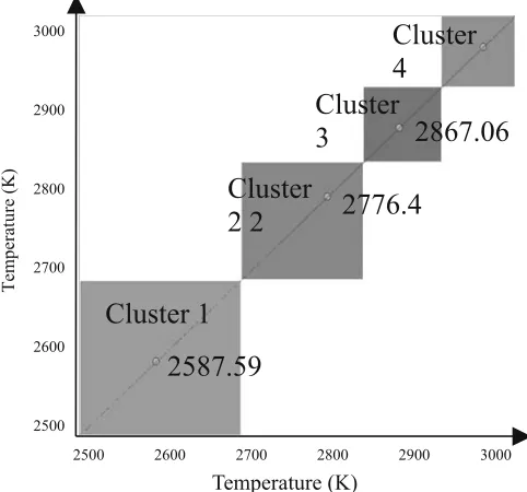
Fig. 5. Clusters of the attribute temperature

consistent and had no null or missing values or errors. Next, the process attributes (parameters) with continuous values (i.e. tem-perature, velocity, and the number of particles) are clustered into four separate ranges using the k-mean clustering algorithm [26]. Clusters of attribute temperature are shown in Fig. 5. Figure 5 depicts the clustering results in two dimensions to illustrate the density of data points in each cluster that are located on the diam-eter. Note that the number of clusters is the choice of the system analyst and determines the number of classes of attributes used in the data mining algorithm. When the choice for the number of clusters is large, each rule generated by the algorithm cov-ers a small number of objects. For example, when the number of clusters is equal to the number of possible attribute values, each rule generated by the algorithm for this attribute will be supported by a single object.

Clustering analysis results for the process attribute tempera-ture are shown in Table 6. Columns 2 and 3 in Table 6 show the range and the mean value of the range for each of the four

Table 6. Four different clusters of attribute temperature

Cluster # Range Mean # Objects

1 [2500, 2684] 2587.59 100

2 [2686, 2820] 2776.4 335

3 [2826, 2915] 2867.06 539

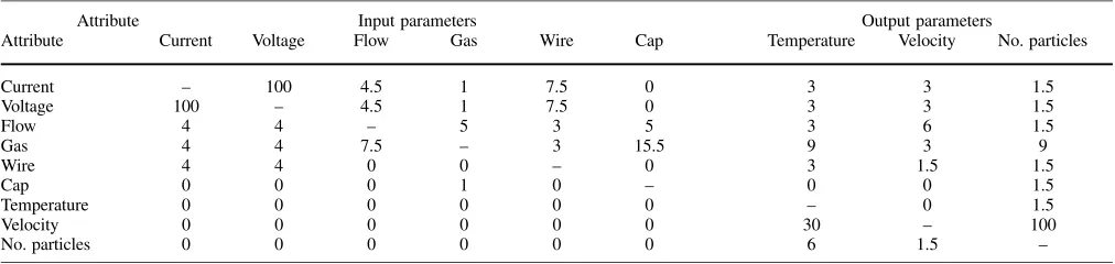
clusters, respectively. Column 4 indicates the number of objects in each cluster. Using a similar clustering approach, values of the attribute velocity and particle number are also grouped into clusters. Once clustering results for these three attributes are ob-tained, continuous values of these attributes are replaced with the corresponding mean values of the clusters in the original dataset. Next, an attribute reduction technique is used to identify and remove the redundant attributes from the dataset. The results of dependency level calculations for all the pairs of attributes of the spray process are summarized in Table 7. From the re-sults in Table 7, it can be seen that the attributes of current and voltage are fully dependent and one of these attributes (i.e. volt-age) can be removed from further analysis without any loss of information.

Once the data preprocessing step is complete, the rule gen-eration algorithm is used to extract useful knowledge from the preprocessed dataset. The rules are used to establish relation-ships between input/output process parameters and to control the output of the spray process. It is important to emphasize that the algorithm allows one to relate multiple input to multiple output

Table 7. Summary of dependency levels calculations

Attribute Input parameters Output parameters

Attribute Current Voltage Flow Gas Wire Cap Temperature Velocity No. particles

Current – 100 4.5 1 7.5 0 3 3 1.5

Voltage 100 – 4.5 1 7.5 0 3 3 1.5

Flow 4 4 – 5 3 5 3 6 1.5

Gas 4 4 7.5 – 3 15.5 9 3 9

Wire 4 4 0 0 – 0 3 1.5 1.5

Cap 0 0 0 1 0 – 0 0 1.5

Temperature 0 0 0 0 0 0 – 0 1.5

Velocity 0 0 0 0 0 0 30 – 100

No. particles 0 0 0 0 0 0 6 1.5 –

Rule 1 IF Gas is N2 THEN Temperature is 2867.06[2826,2915] P=48.8%, Q=98.33%, C=44.17%, QTY=530

Rule 2 IF Current=200 AND Gas is N2 THEN Temperature is 2867.06[2826,2915] P=51.93%, Q=94.99%, C=42.67%, QTY=512

Rule 3 IF Current=200 AND Flow=50 AND Gas is N2 THEN Temperature is 2867.06[2826,2915] P=51.94%, Q=91.84%, C=41.25%, QTY=495

Rule 4 IF Current=200 AND Wire is Solid AND Flow=50 AND Cap Dia. is 0.375 AND Gas is N2 THEN Temperature is 2867.06[2826,2915]

P=59.73%, Q=66.05%, C=29.67%, QTY=356

Rule 5 IF Current=200 AND Wire is Solid AND Flow=50 AND Cap Dia. is 0.375 AND Voltage=32 AND Gas is Arc Jet THEN Temperature is 2963.79[2916,3000]

P=100%, Q=20.35%, C=3.83%, QTY=46

Rule 6 IF Wire is Cored AND Gas is N2 THEN Temperature is 2587.59[2500,2684] P=95.05%, Q=96%, C=8%, QTY=96

Rule 7 IF Current=200 AND Wire is Cored AND Flow=50 AND Cap Dia. is 0.375 AND Gas is N2 THEN Temperature is 2587.59[2500,2684]

P=94.37%, Q=67%, C=5.58%, QTY=67

Fig. 6. Decision rules for the process output temperature

process parameters. The best decision rules obtained from the rule generation algorithm for the control of the average particle temperature of the spray process are shown in Fig. 6.

values of parameters Q and C decrease. Adding another condi-tion attribute to the rule (i.e. Rule 1 versus Rule 2, Rule 2 versus Rule 3, Rule 3 versus Rule 4) makes the rule unique and there-fore parameter P (rule confidence) increases. Clearly, the values of Q and C of the rule are decreasing when the rule is extended to include a new condition parameter. Rule 4 in Fig. 6 may also be considered a strong rule. The condition (i.e.“if”) part of this rule includes all the input parameters of the spray deposition process, and the process output temperature is in the required 2826 K∼2915 K range. The confidence level of Rule 4 is al-most 60% ( P=59.73%), which means that when the process input parameters assume values similar to the ones that appear in the “if” portion of this rule, then 60% of the time a process temperature is between 2826 K and 2915 K. However, only 66% percent of the data records (Q=66.05%) that have a temperature between 2826 K and 2915 K have the values of input parame-ters outlined in Rule 4, and only 29.67% (C=29.67%) of the records of the entire dataset are covered by this rule. Rule 5 is the only rule in which the value of process output temperature is between 1916 and 3000 K. The P value of Rule 5 is 100% (i.e. when the process had input parameters shown in the “if” portion of this rule, the process temperature always fell between 1916 and 3000 K), and it provides the most desirable (highest) outcome for the average particle temperature. However, both the rule support (C=3.83%) and the Q=20.35% value of this rule is very low which implies that the rule is not reliable. Similarly, Rules 6 and 7 have a high confidence (P value), however, due to low support (C value), these rules may not be considered as being reliable for the system analyst.

Rule 1 IF Flow=50 THEN Velocity is 209.6[208.41,211.04] P=51.1%, Q=92.97%, C=45.75%, QTY=549

Rule 2 IF Current=200 THEN Velocity is 209.6[208.41,211.04] P=50.47%, Q=91.71%, C=47%, QTY=564

Rule 3 IF Current=200 AND Flow=50 AND Voltage=32 THEN Velocity is 209.6[208.41,211.04] P=55.39%, Q=85.15%, C=40%, QTY=480

Rule 4 IF Current=200 AND Wire is Solid AND Flow=50 AND Cap Dia. is 0.375 AND Voltage=32 AND Gas is N2 THEN Velocity is 209.6[208.41,211.04]

P=38.09%, Q=53.79%, C=18.92%, QTY=227

Fig. 7. Decision rules for the process output velocity

Rule 1 IF Voltage=32 AND Gas is N2 THEN Velocity is 209.6[208.41,211.04]AND Temperature is 2867.06[2826,2915] P=33.78%, Q=96.53%, C=38.25%, QTY=459

Rule 2 IF Current=200 AND Flow=50 AND Voltage=32 AND Gas is N2

THEN Velocity is 209.6[208.41,211.04]AND Temperature is 2867.06[2826,2915] P=38.78%, Q=88.53%, C=36.25%, QTY=432

Rule 3 IF Current=200 AND Gas is N2 THEN Velocity is 209.6[208.41,211.04]AND Temperature is 2867.06[2826,2915] P=19.78%, Q=96.53%, C=16.25%, QTY=195

Rule 4 IF Current=200 AND Voltage=32 THEN Velocity is 209.6[208.41,211.04]AND Temperature is 2867.06[2826,2915] P=17.97%, Q=97.03%, C=16.33%, QTY=196

Fig. 8. Decision rules for the process output temperature and velocity

Similar analyses are performed for the process output at-tribute of velocity. Figure 7 shows the best decision rules ob-tained from the rule generation algorithm controlling spray pro-cess velocity to be above the desired 200 m/s. Rules 1 and 2 in Fig. 7 provide control of the process velocity with a sin-gle input parameter and have the highest value of (P+Q+ C). However, Rule 3 may be more preferable for the control spray process velocity at levels above 200 m/s. This rule has a higher P value (confidence), an acceptable Q value and the support level is adequate. What is more important is that this rule controls the output velocity of the process with the three different input parameters (current, flow and voltage). Finally, Rule 4 is the best rule for controlling process output velocity with all the input parameters. However, one may see from P, Q, and C values that both the confidence and the support level of this rule is low and as such, the rule cannot be considered reliable.

The analysis presented above suggests that to control average particle temperature of the spray process, Rule 3 in Fig. 6 should be used. According to this rule, when the current is set to 200 A, flow is 50 cfm and N2 gas type is used. In this case, the average particle temperature is above 2700 K. To control average particle velocity, Rule 3 in Fig. 7 should be used. According to this rule, to obtain the average particle velocity above 200 m/s current should be set at 200 A, the flow at 50 cfm and the voltage at 32 V. Finally, if the analyst wants to control both the temperature and the vel-ocity of the spray forming process, then Rule 2 in Fig. 8 should be used. According to this rule, when the current is set to 200 A, flow is 50 cfm, voltage is 32 V and N2-type gas is used. Here, the average particle temperature is above the required 2700 K and the average particle velocity is above the required 200 m/s. One can also see that the input and output parameters of this rule are con-sistent with those of Rule 3 in Fig. 6 and Rule 3 in Fig. 7.

There are two different ways that the knowledge obtained from the data mining algorithm can be used in process control. First, the knowledge (decision rules) can be used by the process analyst to manipulate the spray forming process input attributes to achieve the desired output. It should be noted that when new process data become available, the rules used for process con-trol must be examined for their accuracy and an attempt should always be made to develop new knowledge using this new in-formation. Second, the more desirable approach is the automated process control using the decision rules obtained from the data mining algorithm. Under the scheme of data mining, knowledge generation, and process control, tasks are done automatically. Data obtained from the thermal imaging system is automatically stored in the database and data mining algorithms are used to ex-tract useful knowledge from the dataset. Control software inter-prets the knowledge obtained from the algorithm and automati-cally controls the process input. To implement such an automated control scheme, one needs to develop statistical approaches to ex-amine the validity of each rule generated by the algorithm and to identify the best set of rules for process control. Future research should concentrate both on the development of automated con-trol software and statistical methods that would allow automated process control using the rules generated by the algorithm.

4 Conclusion

In this paper, a new data mining algorithm based on the RS theory was presented for manufacturing process control. The al-gorithm extracts useful knowledge from large datasets obtained from the manufacturing process and represents this knowledge using “if/then” decision rules. An application of the data min-ing algorithm was presented with the industrial example of rapid tool making (RTM). A detailed discussion on how to control manufacturing process output using the results obtained from the data mining algorithm was also presented. Compare to other data mining methods such as decision trees and neural networks, the advantage of the proposed approach is its accuracy, computa-tional efficiency, and ease of use.

References

1. Ruggieri S (2002) Efficient C 4.5. IEEE Trans Knowl Data Eng 14(2):438–444

2. Cantu-Paz E, Kamath C (2003) Inducing oblique decision trees with evolutionary algorithms. IEEE Trans Evol Comput 7(1):54–68 3. Breiman L, Friedman JH (1984) Classification and regression trees.

Wansworth International, Belmont, CA

4. Quinlan JR (1986) Induction of decision trees. Mach Learn 1:81–106 5. Quinlan JR (1993) C4.5: programs for machine learning. Morgan

Kauf-mann, San Mateo, CA

6. Murthy SK (1998) Automatic construction of decision trees from data: a multidisciplinary survey. Data Mining Knowl Discovery 2:345–389 7. Kusiak A (2000) Decomposition in data mining: an industrial case

study. IEEE Trans Electr Packag Manuf 23(4):345–353

8. Mehta M, Agrawal R, Risanen J (1996) SLIQ: a fast scalable classifier for data mining. In: Proceedings of the Fifth International Conference on Extending Database Technology, Avignon, France

9. Shafer J, Agrawal R, Mehta M (1996) SPRINT: a scalable parallel clas-sifier for data mining. In: Proceedings of the International Conference on Very Large Databases, Morgan Kaufmann, pp 544–555

10. Gehrke JE, Ramakrishnan R, Ganti V (2000) RainForest – a framework for fast decision tree construction of large datasets. Data Mining Knowl Discovery 4:127–162

11. Tickle B, Andrews R, Golea M, Diederich J (1998) The truth will come to light: directions and challenges in extracting the knowledge embed-ded within trained artificial neural networks. IEEE Trans Neural Netw 9:1057–1068

12. Lu HJ, Setiono R, Liu H (1996) Effective data mining using neural networks. IEEE Trans Knowl Data Eng 8:957–961

13. Zhang GP (2000) Neural networks for classification: a survey. IEEE Trans Syst Man Cybernetics 30(4):451–462

14. Ripley BD, Ripley RM (1998) Neural networks as statistical methods in survival analysis. In: Dubrowski R, Gant V (eds) Artificial Neu-ral Networks: Prospects for Medicine, Landes Biosciences Publishers, Georgetown, TX, pp 1–13

15. Baxt WG (1995) Applications of artificial neural networks to clinical Medicine. Lancet 346:1135–1138

16. Ostermark R (1997) A fuzzy neural network algorithm for multigroup Classification. Fuzzy Sets Syst 105:113–122

17. Hemsathapat K, Dagli CH, Enke D (2001) Using a neuro-fuzzy-genetic data mining architecture to determine a marketing strategy in a charitable organization’s donor database. In: Proceedings of the IEEE International Engineering Management Conference, Albany, NY, pp 64–69

18. Pawlak Z Rough sets and decision analysis. INFOR 38(3):132–143 19. Pawlak Z (1991) Rough sets – theoretical aspect of reasoning about

data. Kluwer, Dordrecht

20. Pawlak Z (1982) Rough sets. Int J Comput Inf Sci 11:341–356 21. Kusiak A, Kurasek C (2001) Data mining of printed-circuit board

de-fects. IEEE Trans Robot Automat 17(2):191–197

22. Kusiak A, Law IH, Dick M (2001) The G-algorithm for extraction of robust decision rules – children’s postoperative intra-atrial arrhythmia case study. IEEE Trans Inf Technol Biomed 5(3):234–255

23. Ohrn A, Ohno-Machado L, Rowland T (1998) Building manageable rough set classifiers. In: Proceedings of the AMIA Symposium, pp 60–64 24. Kusiak A, Kern JA, Kernstine KH, Tseng BT (2000) Autonomous decision-making: a data mining approach. IEEE Trans Inf Technol Biomed 4(4):274–285

25. Das-Gupta P (1988) Rough sets and information retrieval. ACM Press, New York, pp 567–581

26. Kanungo T, Netanyaho NS, Wu AY (2000) An efficient k-means clus-tering algorithm: analysis and implementation. IEEE Trans Pattern Anal Mach Intell 24(7):887–892

27. Han J, Kamber M (2001) Data mining – concepts and techniques. Mor-gan Kaufmann, San Francisco, CA