5756
AVERAGE AND MAXIMUM WEIGHTS IN WEIGHTED
ROTATION- AND SCALE-INVARIANT LBP FOR
CLASSIFICATION OF MANGO LEAVES
EKO PRASETYO1, R. DIMAS ADITYO2, NANIK SUCIATI3, CHASTINE FATICHAH4
1,2Department of Informatics, Engineering Faculty, University of Bhayangkara Surabaya
Jl. Ahmad Yani 114, Surabaya 60231, Indonesia
3,4Department of Informatics, Information Technology Faculty
Institute of Technology Sepuluh Nopember (ITS) Kampus ITS, Jl. Raya ITS, Sukolilo, Surabaya 60111, Indonesia
Email: 1[email protected], 2[email protected], 3[email protected], 4[email protected]
ABSTRACT
The texture features would be important part when we conduct image classification. Local Binary Pattern (LBP) is one of feature extraction method that has most improvements by many researchers. Weighted Rotation- and Scale-invariant LBP (WRSI-LBP) is one of improvement versions. It uses minimum magnitude of local differences as an adaptive weight (WRSI-LBP-min) to adjust the contribution of LBP code in histogram calculation. The motivation is minimum magnitude gives minimum distortion to change LBP code in histogram calculation. In the classification of mango leaves case, the texture characteristic of mango leaves is highly difficult to be differed directly. So, for high accuracy detection, system requires texture feature with strength discrimination character, robust to illumination change, not sensitive to scaling and rotation. To achieve the goal, we propose average and maximum of magnitude of local differences as an adaptive weight of WRSI-LBP (WRSI-LBP-avg and WRSI-LBP-max). This scheme can be used to generate texture features for classification of mango leaves and general classification cases. The motivation of average weight is to cover all local different magnitude, because each LBP code generated would has unique neighbors pattern. The motivation of maximum is it gives maximum distortion to change LBP code, but it gives highest local different magnitude. We use Support Vector Machine (SVM) and K-Nearest Neighbor (K-NN) as classification methods. We use 240 images for performance evaluation, contains three varieties: Gadung, Jiwo and Manalagi. The K-Fold Cross Validation and Leave-One-Out are used as validation method. From the experiments show that WRSI-LBP-avg and WRSI-LBP-max achieve the highest accuracy compare to WRSI-LBP-min, LBP, Center Symmetric LBP (CS-LBP) and Dominant Rotated Local Binary Pattern (DRLBP). SVM achieve accuracy 75.21% with 16 bins, while K-NN achieve accuracy 79.17% with 256 bins. For uniform pattern, we apply experiments to LBP-min, avg, and max. The highest accuracy is also achieved by avg and WRSI-LBP-max.
Keywords: Texture, Local Binary Pattern, Mango Leaves Classification, Rotation Invariant, Scale
Invariant
1. INTRODUCTION
The texture features would be important part when we conduct image classification. Local Binary Pattern (LBP) is one of feature extraction method that has most improvements by many researchers. The definition of texture had been given by some researcher. Pickett [1] gives statement that texture describe two dimension array of variation, element and arrangement are free but have repetitive characteristic. Hawkins [2] states that the concept of texture is depends on three part, (1) repetitive local ‘order’, (2) element
5757 be guide in parameter measurement of texture slope.
Since Local Binary Pattern (LBP) was introduced by Ojala et al [4], LBP got many improvement to increase performance. Interesting characters of LBP are simplicity, high discrimination, efficient computation, and robust to illumination change. Accompany with its advantages, LBP has some weakness, like sensitive to scaling, rotation, point view variation, amd non-rigid formation. To solve that problems, Davarzani et al [5] proposed Weighted, Rotation- and Scale-Invariant Local Binary Pattern (WRSI-LBP). It isn’t like LBP that regardless magnitude information, which this magnitude is a difference between the central pixel and around neighbors. WRSI-LBP regards difference magnitude as weight. Davarzani et al use minimum difference magnitude between central pixel and around neighbors as the weight used to calculate histogram. The bins used in their experiment research are 256. The reason is minimum difference magnitude gives minimum distortion information. The result of precision classification is 72.32% for Outex dataset. This method needs more research to increase performance.
Some research that concern to leaves detection are Jabal et al [6], his research is plant classification based on leaves feature, Kurniawan et al [7] detect leaves with R-March feature extraction. They make improvements MARCH to be R-MARCH method, so the performance time is shorter. The research in mango leaves detection was published by Prasetyo [8] since 2011. The most important point in this research is that we can detect and know the type of mango tree that has not been fruitful yet. There are three varieties of mango leaves in this research: Gadung, Jiwo, and Manalagi. There are some stage in this research: image acquisition, high light-intensity region separation [9], segmentation [10], feature extraction, and classification. High light-intensity region separation is used to remove high light intensity areas which haven’t true color information. The segmentation is used to separate the objek, mango leaves, from the background. The result of segmentation is uo to 99.5% for segmentation precision. The results of image without high-light intensity area are used in texture generation. The mango leaf texture characteristics among varieties are highly difficult to be differed directly. So, we need a system that can do detection automatically by capture the leaf, process it and give the result. The result of the detection system is the varieties of the mango leaf. In order to doing
detection, we need texture dan color feature. Textures can give local information for leaf surface, while colors can make a difference visually. Some texture schemes has tested to know how big the accuracy is given. We require texture features that can give high accuracy detection, strength discrimination, robust to illumination change, not sensitive to scaling and rotation. Especially for WRSI-LBP, the previous research [5], uses minimum difference magnitude as weight, it doesn’t gives high accuracy in mango leaves detection. For example, in the experiment result in this paper, we get the higher accuracy 73.75% for classification with K-Nearest Neighbor with Leave-One-Out testing. Improvements to the WRSI-LBP method are also important to improve performance when in classification sessions. So, we need a modification for this scheme in order to get higher accuracy. In this research, we try to use average and maximum magnitude difference as weight to calculate histogram in WRSI-LBP, in order to exchange minimal magnitude difference. The motivation of average weight is to cover all local different magnitude, because each LBP code generated would has unique neighbors pattern. The motivation of maximum is it gives maximum distortion to change LBP code, but it gives highest local different magnitude. In the classification stages, we use Support Vector Machine (SVM) and K-Nearest Neighbor (K-NN) as classification methods. For experiment, we have 240 images for performance evaluation, contains three varieties: Gadung, Jiwo and Manalagi. The K-Fold Cross Validation and Leave-One-Out are used as validation method.
2. BASIC LBP AND ITS IMPROVEMENTS
5758 middle right side neighbor, then move around clockwise, as presented in Fig. 2.
Figure 1: Basic LBP, (a) 3x3 Neighborhood system; (b) Thresholded by center value; (3) Weighted matrix
Figure 2: Circularly symmetric neighborhood with radius R and P neighborhood pixel
Let I(x,y) is gray level image, and gc is
gray level of any pixel position (xc,yc), for example
gc=I(xc,yc). Gray level value of the P is around
neighbor used by all image pixel, with around neighbor at radius R (R>0), around gc is gp, p = 0,
1,…,P-1. Standard form of LBPP,R(xc,yc) is
explained below. 1 ,..., 0 ), , (
I x y p P
gp p p
) / 2
cos( p P
R x
xp c
) / 2cos( p P
R y
yp c
1
0
, ( , ) ( )2
P p p c p c c R
P x y s g g
LBP 0 , 0 0 , 1 ) ( x x x
s (1)
According to the Eq. (1), if the block in the image is rotated then the around neighbor of central pixel would be moved too. To achieve rotation invariance, basic LBP code is rotated according to minimum value [4] using Eq. (2).
( , )| 0,1..., 1
min ,
, RORLBP i i P
LBPPriR PR (2)
Where superscript “ri” is “rotation invariance”. Function ROR(x,i) rotates P bit binary number x amount i times to the right direction (IiI<P).
3. WEIGHTED ROTATION- AND
SCALE-INVARIANT LBP (WRSI-LBP)
Davarzani et al [5] proposed a scheme to solve a problem where LBP disregards magnitude of local different when it computes histogram. This weighting scheme is accompany with the Rotation- and Scale-invariant LBP (RSI-LBP) and make a complete scheme, Weighted Rotation- and Scale-invariant LBP (WRSI-LBP). Next we would discuss about it.
The scheme of basic LBP operator, each central pixel is calculated LBP value by compare it with around neighbors in a fixed R radius before. So, if the image is rescaled, the neighbor’s pixel around the central pixel will be changed and produce different LBP code. This causes basic LBP features are not invariant to scaling transformation [5]. By using local maxima of the Laplacian of Gaussian (LoG) measure in the scale-space, we can improve LBP descriptor as an adaptive scale [5]. For different levels of the scale-space representation of an image is defined as a function, L(x,y,σ). This is result of convolution image I(x,y) by a variable-scale Gaussian, G(x,y,σ).
) , ( ) , , ( ) , ,
(x y G x y I x y
L
(3)) 2 / ) (( 2 2 2 2 2 1 ) , , (
e x yy x
G (4)
Therefore, using a scale-adaptive local binary pattern a high degree of scale invariance could be achieved [5]. The maximum result of from
| ) , , ((
|LoG x y
with scale σ = 1,2,…,N is selected as the characteristic scale, Eq. (5).N y x L y x L y x
LoG xx yy
..., 2 , 1 , ) , , ( ) , , ( ) , , ( 2
2 2 2 2 , y L L x LLxx yy
(5)
Then, r(x,y)
is assigned as the circular neighboring set of the image pixel (x,y) in the LBP equation. The modified of basic LBP become as follows:1 ,..., 0 ), , (
I x y p P
gp p p
) / 2 cos( ) ,
(x y p P
r x
xp c c c
) / 2 sin( ) ,(x y p P
r y
yp c c c
1 0 ) , (, ( , ) ( )2
P p p c p c c y x R
P x y s g g
LBP c c (6)
5759 invariant problem, where LBP code resulted from degree 0o is different from other degrees [5].
Figure 3: Dominant orientation assignment in gc [5]
Davarzani et al [5] proposed WRSI-LBP to solve rotation invariant by determine start point of each LBP code adaptively. An orientation value is assigned to each central pixel and LBP operator is represented relatively to the assigned orientation value. The dominant orientation is computed by the dominant gradient orientation value direction. Fig. 3 show example of orientation assignment process for the central pixel, gc, In order to perform all
computation in scale-invariant manner, for each central pixel, gc, its characteristic scale σc is used to
create Gaussian smoothed image, L(x,y, σc). For
each image sample, L(x,y, σc), in the region around
the central pixel, gc, pixel differences are used to
calculated its gradient magnitude, m(x,y), and orientation θ(x,y):
2
2 ( ( , 1) ( , 1))
)) , 1 ( ) , 1 ( ( ) , ( y x L y x L y x L y x L y x m ) , 1 ( ) , 1 ( ) 1 , ( ) 1 , ( tan ) , ( 1 y x L y x L y x L y x L y x
(7)
After that, an orientation histogram of local gradient angles is generated. It has hb bins
representing the 360o range of possible orientation
degree. Each point is weighted by Gaussian-weighted circular window function, then it is added to the histogram. The Gaussian-weighted circular window function use Gaussian kernel RG centered on gc. RG is a multiple of the characteristic scale in
gc. The highest peak in this histogram corresponds
to dominant direction of local gradients and is selected as pixel’s orientation.
Let θc be assigned to the central pixel gc =
(xc,yc), so, gray value of P equally spaced circular
neighborhood pixels on a circle of radius R(R>0), surround gc can be determined by equation:
1 ,..., 1 , 0 ), , (
I x y p P
gp p p
) / 2
cos( c
c
p x R p P
x
) / 2
sin( c
c
p y R p P
y
(8)Davarzani et al show example for the scheme of rotation adaptive LBP [5]. After get the patch image, in the region around central pixel, the corresponding gradient of each central pixel is computed. The local gradient orientations of neighbor within the region of the central pixel are accumulated into a histogram. The largest bin of orientation in the histogram is selected as dominant orientation. Therefore, orientation θc is assigned to
this pixel, gp, p=0,1,…,7 are located using Eq. (8).
Afterthat, start from the neighbor with p=0, then go to p=1, etc., use as weighted LBP code.
In the basic LBP, histogram is calculated regardless the magnitude of local different between central pixel and the around neighbor (Eq. (1)). Davarzani et al give a scheme, we use simple weighting to incorporate magnitude information into LBP histograms. In a local neighborhood, magnitude value between central pixel with one local neighbor dan others is different. The proximity of neighboring pixels to central pixel in uniform parts of the image produces small different magnitude. The basic LBP only uses the sign of local differences with the same weight to each LBP pattern. While the WRSI-LBP regard the differences.
The motivation of weighting scheme is to assign the magnitude of local differences as strength of corresponding bits in the LBP code. The magnitude of each bit in LBP code can be considered as a measure which shows its robustness [5]. The stability of each LBP code depends on the strength of its constituent bits separately. To give the impact of each LBP code in to the feature histogram, the minimum distortion to change LBP code is considered as weight measure. The minimum magnitude of local differences is considered as the minimum distortion. Therefore, in WRSI-LBP, the minimum magnitude of local differences as an adaptive weight to adjust the contribution of LBP code in histogram calculation. Each LBP code is added to the LBP histogram by weighting with its minimum value of different magnitude [5]. Suppose the texture image is N x M and the LBP pattern of each pixel (I,j) is denoted as
) , ( , i j
LBPPR . The weighted LBP (WLBP) histogram is computed as :
N i M j R P RP h w LBP i j h h H
WLBP
1 1
,
, ( ) ( (, ), ), 0,
5760 where, H is the maximal LBP pattern value.
This weight scheme is used in WRSI-LBP and is conducted on some selected public dataset, such Outex [13], Brodatz [14], UIUC [15], and UMD [16] datasets.
4. PROPOSED WEIGHT VARIANCE OF
WEIGHTED ROTATION- AND SCALE-INVARIANT LBP (WRSI-LBP)
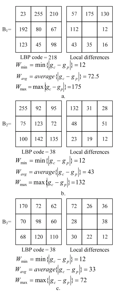
Although minimum value of local different magnitude gives minimum distortion to change LBP code, it doesn’t regard local different magnitude among neighboring pixel and the central pixel. Some pattern of unique case in LBP code can’t be covered. Fig. 4 gives example. For convenience, we give illustration weighting scheme in basic LBP, but we can use this weighting scheme in all LBP variance. From that figure example, B1
and B2 are two case of central pixel that we would
calculate the weight. For B1, and B2, we get LBP
code 218, and 38 respectively, but each has same weight in Min weighted scheme, 12. Although, this gives minimum distortion to change LBP code, but each gives same weight in histogram calculation. That causes histogram would be alike with without weight. For B2, and B3, we get same LBP code, 38,
we get same weight too, 12. It should be each has different weight for each case of pattern. We need a weight scheme that can cover different weight on different LBP code depends to local different magnitude.
We propose average value of local different magnitude as new weight scheme in weighted LBP. The motivation of weighting scheme with the average is to cover all local different magnitude, because each LBP code generated would has pattern of its neighbors. Therefore, by calculated average of local different magnitude, we would capture a pattern from each LBP code depends on around neighbors. As presented on Fig. 4, B1 and B2, have different LBP
code, and get different weight by average of local different magnitude, 72.5 and 43, respectively. For B2 and B3, although have same LBP code, 38, they
have different weight, 43 and 33, respectively. In this paper, we also propose weighted LBP by maximum value of local different magnitude as other optional weighting scheme. The motivation of maximum is it gives maximum distortion to change LBP code, but it gives highest local different magnitude and gives maximum distortion to change LBP code.. As presented in Fig. 4, B1, B2, and B3 have different maximum
value of local different magnitude, but sometime it
doesn’t possible will has same value. We would use average and maximum value of local different magnitude that compared to other scheme of LBP, as we would discuss at next part.
12 } min{
min gcgp
W
5 . 72 }
{
c p
avg average g g
W
175 } max{
max gcgp
W
12 } min{
min gcgp
W
43 }
{
c p
avg average g g
W
132 } max{
max gcgp
W
12 } min{
min gcgp
W
33 }
{
c p
avg average g g
W
72 } max{
max gc gp
[image:5.612.319.516.142.645.2]W
Figure 4: Local different magnitude between the central pixel and around neighbor with some selected weighting
5761
5. EXPERIMENT IN MANGO LEAVES
CLASSIFICATION
Research field in mango leaves varieties classification would be a deep challenge when we detect on not yet-fruitful mango leaves based on leaf, as presented by Prasetyo [8], in [9] we would detect mango leaves varieties based on color, texture and shape of leaf. This research has started from last several years [17], and has some experience testing. To avoid high light-intensity on leaf region of image, we have to detect it and remove from image, as presented in [9]. Removing of high light-intensity on leaf region is conducted after segmentation result. Then, some features would be extracted, such mean and standard deviation of color, LBP, compactness and circularity. Especially for LBP, we would use improved version of WRSI-LBP with average weight.
We conducted experiment on 240 images of mango leaf. We use three varieties of mango leaves, Gadung, Jiwo, and Manalagi. For each mango leaf variety, we have 80 leaves as sample. We use mango leaf region that high light-intensity on leaf region was removed. Then we generate WRSI-LBP with average weight (WRSI-LBP-avg) and WRSI-LBP with maximum weight (WRSI-LBP-max) to the histogram result, each gives 256 bins.
We also generate some LBP-based features, such basic LBP [4], Center Symmetric LBP (CS-LBP), Dominant Rotated Local Binary Pattern (DRLBP) [18]. WRSI-LBP with minimum weight (WRSI-LBP-min). Then we compare their performance on both Support Vector Machine (SVM) and K-Nearest Neighbor (K-NN). For SVM, we use Linear as kernel function applied, for K-NN we use 1 neighbor as nearest neighbor. Especially for K-NN, dissimilarity between two histograms has to use appropriate distance. As presented by Davarzani et al [5], distance measurement of two histograms may be conducted with histogram intersection, log-likelihood ratio, or chi-square statistic. And we use chi-square statistic as distance between two histograms. In out experiment, we also conducted performance comparison on Uniform pattern of WRSI-LBP-min, WRSI-LBP-avg, and WRSI-LBP-max. So we can give a comprehensive analyzing of WRSI-LBP scheme comparison.
The result of our experiment is presented below. We conducted testing on several numbers of bin, such 256, 128, 64, 32, and 16. Especially for CS-LBP, it just apply to 16 bins. For all our testings, we conducted by K-Fold Cross validation
with K=5, so for every session testing, we use 20% data as training data, and 80% data as testing data. And then we calculate average accuracy from 5 session testing of K-Fold. Except for K-NN as presented on part 4.3, we use Leave-One-Out as testing method.
5.1 Testing Result on SVM
We conducted testing on SVM with kernel function Linear, the result is presented on Table 1 below. Our problem is multiclass, so we use SVM Multiclass problem [19] with Error Correcting Output Code approach. From data presented on Table 1, the highest accuracy is given by WRSI-LBP-avg with value 73.44% at bin 32. From the other bins used, the highest accuracy is also given by WRSI-LBP-avg, except for bin 128, the highest accuracy is given by WRSI-LBP-max. While for bin 64, WRSI-LBP-avg and WRSI-LBP-max get highest accuracy. Actually, the accuracy result from WRSI-LBP schemes have more accuracy significantly compared to other LBP schemes, but min, avg and WRSI-LBP-max can improve accuracy. Although we decrease number of bins, the accuracy of WRSI-LBP can hold accuracy over 70%.
Table 1. Accuracy (%) prediction from testing result on SVM
Method 256 128 Bin 64 32 16
LBP 66.56 66.46 67.29 62.08 64.17
CS-LBP - - - - 68.23
DRLBP 62.08 64.38 57.50 57.40 58.13
WRSI-LBP-min 65.63 66.04 67.29 70.42 72.29
WRSI-LBP-avg 69.06 71.04 71.15 73.44 75.21
WRSI-LBP-max 68.85 71.67 71.15 73.23 74.79
5.2 Testing Result on Nearest Neighbor with K-Fold Cross Validation
WRSI-LBP-5762 avg and WRSI-LBP-max can improve accuracy, and hold over 70%, while the others below 70%.
When we try to improve number of K in K-NN with 3, we get all accuracy from method used get down below 70%, the highest accuracy is 62.19% by WRSI-LBP-avg with 128 bins. As presented on Table 3. But from all bins used, all highest accuracy are given by WRSI-LBP-avg.
Table 2. Accuracy (%) prediction from testing result on K-NN with K=1, distance is Chi-Square, and K-Fold
Cross Validation
Method 256 128 Bin 64 32 16
LBP 70.52 69.90 69.90 68.02 65.94 CS-LBP - - - - 68.96 DRLBP 65.31 66.98 64.48 66.25 65.83
WRSI-LBP-min 70.42 70.42 69.48 72.92 69.90
WRSI-LBP-avg 71.46 74.17 72.50 73.33 71.25
[image:7.612.91.299.213.343.2]
WRSI-LBP-max 71.04 73.13 71.15 72.71 72.08
Table 3. Accuracy (%) prediction from testing result on K-NN with K=3, distance is Chi-Square, and K-Fold
Cross Validation
Method 256 128 Bin 64 32 16
LBP 56.25 58.33 57.29 52.60 55.94
CS-LBP - - - - 57.29
DRLBP 51.46 56.35 52.60 52.92 55.31
WRSI-LBP-min 56.35 58.54 57.40 55.83 56.25
WRSI-LBP-avg 60.10 62.29 61.25 59.17 61.04
WRSI-LBP-max 59.79 61.67 59.90 59.17 60.73
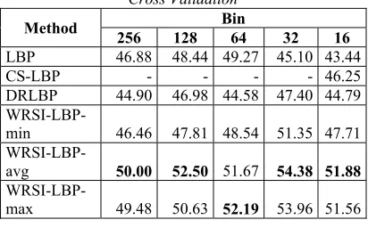
Table 4. Accuracy (%) prediction from testing result on K-NN with K=5, distance is Chi-Square, and K-Fold
Cross Validation
Method 256 128 Bin 64 32 16
LBP 46.88 48.44 49.27 45.10 43.44
CS-LBP - - - - 46.25
DRLBP 44.90 46.98 44.58 47.40 44.79
WRSI-LBP-min 46.46 47.81 48.54 51.35 47.71
WRSI-LBP-avg 50.00 52.50 51.67 54.38 51.88
WRSI-LBP-max 49.48 50.63 52.19 53.96 51.56
We also try to improve number of K in K-NN with 5, we get all accuracy from method used also get down below 60%, the highest accuracy is 54.38% by WRSI-LBP-avg with 32 bins. As presented on Table 4. But from all bins used, all
highest accuracy are given by WRSI-LBP-avg, except for 64 bins, the highest accuracy is given by WRSI-LBP-max.
5.3 Testing Result on Nearest Neighbor with Leave-One-Out
To prove our conclusion next, we conducted a performance comparison to selected method with a testing by Leave-One-Out. In this testing, we use 1 data as testing data, while the rest would be training data. With Leave-One-Out, we have some advantages, such we use maximum training data, and we conducted testing with high variance of result.
Table 5. Accuracy (%) prediction from testing result on K-NN with K=1 and distance is Chi-Square and
Leave-One-Out
Method 256 128 Bin 64 32 16
LBP 70.42 73.33 71.25 69.58 70.83
CS-LBP - - - - 73.75
DRLBP 74.58 69.58 71.67 67.92 62.92
WRSI-LBP-min 71.67 73.33 73.75 73.33 71.25
WRSI-LBP-avg 77.92 77.92 78.33 75.83 76.25
[image:7.612.91.297.369.509.2]WRSI-LBP-max 79.17 78.75 77.92 74.17 75.00
Table 6. Accuracy (%) prediction from testing result on K-NN with K=3 and distance is Chi-Square and
Leave-One-Out
Method Bin
256 128 64 32 16
LBP 65.00 65.83 65.42 66.25 67.50
CS-LBP - - - - 66.67
DRLBP 57.08 57.92 57.92 62.50 58.33
WRSI-LBP-min 61.25 62.92 60.42 62.08 63.75
WRSI-LBP-avg 61.67 66.67 65.83 67.08 71.25
WRSI-LBP-max 62.50 64.17 63.33 67.50 67.92
Table 7. Accuracy (%) prediction from testing result on K-NN with K=5 and distance is Chi-Square and
Leave-One-Out
Method 256 128 Bin 64 32 16
LBP 60.83 60.83 61.67 57.92 58.33
CS-LBP - - - - 58.33
DRLBP 47.50 47.92 49.58 54.17 52.50
WRSI-LBP-min 53.33 53.75 55.83 55.42 58.33
WRSI-LBP-avg 57.08 60.00 59.58 62.08 65.42
[image:7.612.92.298.534.662.2]
5763 We conducted on K-NN with K=1, K=3, and K=5. All testing result presented on Table 5, 6, and 7. Generally, the accuracy performance always decreases as long as we increase number of K, same as previous result. In this result, the highest accuracy of K=1 is 79.17%, using WRSI-LBP-max with 256 bins is shown Table 5. While the highest accuracy of K=3 is 71.25%, using WRSI-LBP-avg with 16 bins is shown Table 6. And the highest accuracy of K=5 is 65.42%, using WRSI-LBP-max with 16 bins is shown Table 7.
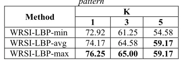
5.4 Testing Result on Nearest Neighbor with Uniform Pattern
[image:8.612.101.289.360.422.2]Based on uniform pattern from Ojala et al [4], we conducted testing on uniform pattern only. Uniform patterns get 58 bins for each WRSI-LBP scheme. We generate uniform pattern from previous LBP (LBP-min), WRSI-LBP-avg, and WRSI-LBP-max. The result is presented by Table 8.
Table 8. Accuracy (%) prediction from testing result on K-NN and distance is Chi-Square and K-Fold on uniform
pattern
Method 1 K 3 5
WRSI-LBP-min 72.92 61.25 54.58 WRSI-LBP-avg 74.17 64.58 59.17 WRSI-LBP-max 76.25 65.00 59.17
From the the result above, the highest accuracy always are achieved by WRSI-LBP-max, both on K=1, K=2, and K=3. For K=5, WRSI-LBP-avg and WRSI-LBP-max get the highest accuracy.
In our experiments, it was presented that WRSI-LBP-avg and WRSI-LBP-max give highest accuracy in K-NN classification for mango leaf detection. Although both methods aren’t present the minimum distortion because it isn’t minimum magnitude of local differences. But WRSI-LBP-avg takes average weight from local difference magnitude between central pixel and around neighbors, so it considers all the difference magnitude. While WRSI-LBP-max take the maximum distortion and sometimes it gives highest accuracy. Generally, both WRSI-LBP-avg and WRSI-LBP-max give the higher result in classification of mango leaf varieties compare to previous WRSI-LBP (WRSI-LBP-min) and the others.
6. CONCLUSIONS
This research has done experiment in modification of WRSI-LBP to improve
performance. Using average of local difference magnitude as weight in WRSI-LBP-avg and using Chi-Square distance, we can improve accuracy significantly. For the SVM classification, we get highest accuracy of WRSI-LBP-min 75.21% compare to previous WRSI-LBP 72.29%. Also in K-NN classification, we get highest accuracy of WRSI-LBP-max 78.75% compare to previous WRSI-LBP 73.33%. The characteristic of texture features of mango leaf varieties have similar character, but by average and maximum weight in WRSI-LBP we can improve some weakness of WRSI-LBP
We just test this method on SVM and K-NN for classification in order to prove performance improvement, for next result, need a testing on some other classification method. We also require a testing on some other public dataset, so we can get comparing result of these weighting scheme.
ACKNOWLEDGMENT
The authors give thanks to the Directorate of Research and Community Service (DRPM) DIKTI that fund Authors’ research in the scheme of Inter-Universities Research Cooperation (PEKERTI) year 2017 between University of Bhayangkara Surabaya and Institute of Technology Sepuluh Nopember, with contract number 010/SP2H/K2/KM/2017, on 4 May 2017.
REFERENCES:
[1] R. M. Pickett, Visual Analysis of Texture in the Detection and Recognition of Objects. New York: Academic Press, 1970.
[2] J. K. Hawkins, Textural Properties for Pattern Recognition. New York: Academic Press, 1970.
[3] W. K. Pratt, Digital Image Processing. Hoboken, New Jersey: John Wiley & Sons, 2007.
[4] T. Ojala, Pietikainen, M., Maenpaa, T., "Multiresolution gray-scale and rotation invariant texture classification with local binary pattern," IEEE Transaction Pattern Analysis and Machine Intelligence, vol. 24, pp. 971-987, 2002.
[5] R. Davarzani, Mozaffari, S., Yaghmaie, K., "Scale- and rotation-invariant texture description with improved local binary pattern features," Signal Processing, vol. 111, pp. 274-293, 2015.
5764 Computer Science, vol. 9, pp. 1295-1304, 2013.
[7] M. G. Kurniawan, Suciati N., and Fatichah C., "Sistem Temu Kembali Citra Daun Menggunakan Metode Reduced Multi Scale Arch Height (R-March) Pada Smartphone," JUTI, vol. 4, pp. 145-153, 2016.
[8] E. Prasetyo, "Detection of Mango Tree Varieties Based on Image Processing," Indonesian Journal of Science & Technology, vol. 1, pp. 203-215, 2016.
[9] E. Prasetyo, Adityo, R.D., Suciati, N., and Fatichah, C., "Deteksi Wilayah Cahaya Intensitas Tinggi Citra Daun Mangga Untuk Ekstraksi Fitur Warna dan Tekstur Pada Klasifikasi Jenis Pohon Mangga," presented at the Seminar Nasional Teknologi Informasi, Komunikasi dan Industri, UIN Sultan Syarif Kasim Riau, 2017.
[10] E. Prasetyo, Adityo, R.D., Suciati, N., and Fatichah, C., "Mango Leaf Image Segmentation on HSV and YCbCr Color Spaces Using Otsu Thresholding," in International Conference on Science and Technology, Yogyakarta, 2017.
[11] Z. S. Tang, Y., Er M.J., Qi, F., Zhang, L., Zhou, J., "A local binary pattern based texture descriptors for classification of tea leaves," Neurocomputing, vol. 168, pp. 1011-1023, 2015.
[12] C. Silva, Bouwmans, T., Frelicot, C., "An eXtended Center-Symmetric Local Binary Pattern for Background Modeling and Subtraction in Videos," presented at the International Joint Conference on Computer Vision, Imaging and Computer Graphics Theory and Applications, Berlin, Germany, 2015.
[13] T. Ojala, Mäenpää, T., Pietikäinen, M., Viertola, J., Kyllönen, J., and Huovinen, S., "Outex - new framework for empirical evaluation of texture analysis algorithm," presented at the Proceedings of the International Conferenceon Pattern Recognition, 2002.
[14] P. Brodatz, "Textures: A Photographic Album for Artists and Designers," ed. Dover, New York, 1966.
[15] S. Lazebnik, Schmid, C., and Ponce, J., "A sparse texture representation using local affine regions," IEEE Transact. Pattern Anal. Mach. Intell., vol. 27, pp. 1265-1278, 2005.
[16] X. Yong, Xiong, Y., Haibin, L., and Hui, J., "A new texture descriptor using multifractal analysis in multi-orientation wavelet pyramid," in IEEE Conferenceon Computer Vision and Pattern Recognition (CVPR), 2010, pp. 161-168.
[17] S. Agustin, and Prasetyo, E., "Klasifikasi Jenis Pohon Mangga Gadung Dan Curut Berdasarkan Tesktur Daun," in Seminar Nasional Sistem Informasi Indonesia, Surabaya, 2011.
[18] R. Mehta, and Egiazarian, K., "Dominant Rotated Local Binary Patterns (DRLBP) for Texture Classification," Pattern recognition Letters, vol. 71, pp. 16-22, 2016.
![Figure 3: Dominant orientation assignment in g c [5] Davarzani et al [5] proposed WRSI-LBP](https://thumb-us.123doks.com/thumbv2/123dok_us/8905740.956734/4.612.138.249.129.230/figure-dominant-orientation-assignment-davarzani-proposed-wrsi-lbp.webp)