A semi analytical lagrangian model to simulate the contaminants dispersion in the stable boundary layer

Full Length Research Article

A SEMI-ANALYTICAL LAGRANGIAN MODEL TO SIMULATE THE CONTAMINANTS DISPERSION IN

THE STABLE BOUNDARY-LAYER

1,*

_{Jonas C. Carvalho,}

2

_{Daniela Buske and}

2

_{Régis S. de Quadros}

1

_{Universidade Federal de Pelotas, Faculdade de Meteorologia, Programa de}

Pós-Graduação em Modelagem Matemática, Pelotas, Brazil

2

_{Universidade Federal de Pelotas, Instituto de Física e Matemática, Programa de}

Pós-Graduação em Modelagem Matemática, Pelotas, Brazil

ARTICLE INFO ABSTRACT

A semi-analytical solution for the three-dimensional Langevin equation is presented and used to study the contaminant dispersion in the Stable Boundary-Layer (SBL). The method leads to a stochastic integral equation whose solution is based on the iterative solution of Langevin equation by the Picard’s Iterative Method. The novelty in this work relies on the consideration of the Eulerian autocorrelation function suggested by Frenkiel (1953) and Murgatroyd (1969). By this procedure the method is able to simulate the pollutant dispersion in the SBL for low wind and windy conditions, depending on the parameter associated with the characteristic period due the meander. The numerical simulations and comparisons with measured data performed shows a good agreement between predicted and observed values.

Copyright©2016,Jonas C. Carvalho et al. This is an open access article distributed under the Creative Commons Attribution License, which permits unrestricted use, distribution, and reproduction in any medium, provided the original work is properly cited.

INTRODUCTION

The study of the Stable Boundary-Layer (SBL) over land under fair weather conditions is of major concern in air pollution meteorology. Most of the industrial stacks are located within this layer and hence the dispersion of air pollutants is adversely affected by the state of the SBL (Sharan and Gopalakrishnan, 2003). The mathematical modelling of the SBL has encountered difficulties in several aspects, mainly because of either the low intensity of the turbulent energy and phenomena such as meandering, which happens when the mean wind velocity approaches zero. In fact, dealing with turbulence and atmospheric dispersion studies, low wind speeds are generally considered the most critical conditions. Under low wind conditions, horizontal diffusion is enhanced due the meander and the resulting ground-level concentration is generally much lower than that predicted by traditional techniques, becoming their application limited and (Oettl et al., 2001; Anfossi et al., 2005). Turbulent dispersion of scalars is probably best understood in a Lagrangian framework as first suggested by Taylor´s statistical theory of dispersion in homogeneous turbulence (Weil et al., 2004). Lagrangian particle models are an important and effective tool to simulate the atmospheric dispersion of airborne pollutants. These models are based on the Langevin equation, which is derived from the hypothesis that the velocity is given by the combination between a deterministic and a stochastic term. The main advantages of these models in relation to the other techniques (similarity or gradient-transfer theory) are the simplicity, flexibility and the ability to incorporate temporal and spatial variations in turbulence properties (Luhar and Britter, 1989; Shankar Rao, 1999). As a consequence, important features of flow and turbulence fields (such as the vertical profiles of wind speed, standard deviation and higher order moments of wind speed fluctuation) can be included in the model, thus allowing a more accurate simulation without consuming excessive computer time.

*Corresponding author: Jonas C. Carvalho,

Universidade Federal de Pelotas, Faculdade de Meteorologia, Programa de Pós-Graduação em Modelagem Matemática, Pelotas, Brazil.

ISSN: 2230-9926

International Journal of Development Research

Vol. 06, Issue, 11, pp.10371-10379, November,2016

DEVELOPMENT RESEARCH

Article History:

Received 29th _{August, 2016}

Received in revised form 17th _{September, 2016}

Accepted 08th _{October, 2016}

Published online 30th _{November, 2016}

Key Words:

Currently, the search for analytical solutions for the dispersion problems is one of the main research subjects in the pollutant dispersion modelling. These solutions become important due to the intention to obtain dispersion models that generate reliable results in a small computational time to be used in regulatory air pollution modelling. Analytical solutions, being the influencing parameters explicitly expressed in a mathematical closed form, allow in general a deep sensitivity analysis over model parameters. Moreover, computer codes based on analytical expressions in general do not have prohibitive computational resources.

In this work a Lagrangian particle model is proposed to investigate the contaminant dispersion in stable conditions. The model is based on the methodology proposed in three recent papers by Carvalho et al. (2005 a,b; 2013), which solves the Langevin equation, in semi-analytical manner, by the Method of Successive Approximations or Picard’s Iterative Method. The novelty of this work relies on the consideration of the Eulerian autocorrelation function suggested by Frenkiel (1953) and Murgatroyd (1969) in the equations of the turbulent velocities. The autocorrelation function suggested by Frenkiel (1953) and Murgatroyd (1969) generates a negative lobe for the horizontal wind components attributed to the meander. By considering this formulation, it is now possible to show the aptness of this method to simulate the pollutant dispersion in the SBL during low wind and higher wind speeds, setting the value of the parameter associated with the characteristic period of the oscillation due the meander. The proposed approach is called Iterative Langevin Solution (ILS). To evaluate the ILS approach, the data collected during the stable conditions conducted at the Idaho National Engineering Laboratory (INEL) (Sagendorf and Dickson, 1974) and during stable Prairie Grass tracer experiment (Barad, 1958) have been used. The paper is outlined as follows: in section two we present the Iterative Langevin Solution, in section three we show the turbulent parameterisation, in section four we report the results and in section five we present the conclusions.

Iterative Langevin Solution (ILS)

ILS is an alternative numerical solution for the Langevin equation, which consists in an iterative solution by the Picard Method. Based on this numerical solution, the contaminant dispersion consists in the linearization of the Langevin equation as stochastic differential equation:

 

t

U

g

 

t

f

dt

dU





, (1)

which has the well known solution in terms of the integrating factor

 t t dt t f e0 ' '₎ ( : ' ) ( ' ) ( 0 0 ' ' 0 ' ' ) ( 1 dt e t g e U t t dt t f dt t f t t t t



  

. (2)

In order to embody the low wind speed condition in the Langevin equation, it is assumed that

U

and

f

(

t

)

are complex functions written as:

iv

u

U





₍₃₎

and

 

t

p

iq

f





, (4)

where

u

and

v

are the real and imaginary parts of

U

, respectively, and

p

and

q

are the real and imaginary parts of

f

(

t

)

, respectively. Therefore, the exponentials appearing in Equation (2) reads like:

iqt pt dt t f

e

e

t

t0

_



'

'₎

(

. (5)

Applying the Euler formula, Equation (2) becomes:

          

 

' ' ' ' 0 ' )] ( ) [cos( 1 sin cos 0 0 ) ( ) cos( dt qt sin i qt e t g qt i qt e iv u qt sin i qt e U t t pt pt pt                  

. (6)

Multiplying the Equation (6) by the complex conjugate and performing the multiplications, we can obtain

Considering

t



t







, we can write the Equation (7) as



_{cos( ) ( )}





 

₀

 

₀



 

'



_cos

 

_sin

 



'

0 dt q i q e t g iv u qt sin i qt e U t t p

pt _{     }

  _  

(8)

In order to determine the wind direction we recast equation (8) like:

 

₀

 

'



_cos

 



' _{sin( )}

 

₀

 

'



_sin

 



'

) cos( 0 0 dt q e t g v qt e dt q e t g u qt e U t t p pt t t p

pt _{    }

  _    _  

, (9)

where by comparison with Equation (3) we have

 

₀

 

'



_cos

 



'

)

cos(

0

dt

q

e

t

g

u

qt

e

u

t t p

pt

_

_





_

 

(10a) and

 

₀

 

'



_sin

 



'

)

sin(

0

dt

q

e

t

g

v

qt

e

v

t t p

pt

_

_





_

 

. (10b)

The Equation (9) is a non-linear stochastic integral equation, which must be solved iteratively. The method applied to solve the Equation (9) is the Method of Successive Approximations or Picard’s Iteration Method (Boyce and DiPrima, 2001), assuming that the initial guess for the iterative approximation is determined from a Gaussian distribution. Bearing in mind the isomorphism between the complex and real planes, we promptly realize that the low wind expression given by Equation (9) is described in the complex plane. This procedure allows to determine the low wind direction, using polar form. For such, we rewrite Equation (9) like







u

v

e

i

U

2 2 _,

(11) where



is the low wind direction relative the x-axis

















u

v

arctan

(12)

Now, giving a closer look to the real component of the Equation (9), we realize that



 





 

q

e

p

cos

_{is analogous to the Eulerian}

autocorrelation function suggested by Frenkiel (1953, p. 80) and written in a different way by Murgatroyd (1969). Therefore,

p

and

q

are given by

T

m

p

)

1

(

1

2





and

m

T

m

q

)

1

(

2





where

T

is the time scale for a fully developed turbulence and

m

is a non-dimensional quantity that controls the meandering oscillation frequency. The autocorrelation function suggested by Frenkiel (1953) and Murgatroyd (1969) generates a negative lobe for the horizontal wind components attributed to the meander. Following Anfossi et al. (2005), it is important to notice two important situations. When

m



0

, the dispersion in the SBL is under meandering effect, which occur during low wind conditions. In this case, Equation (9) is written in terms of the Frenkiel (1953) and Murgatroyd (1969) autocorrelation function. When

m



0

, the meandering effect is eliminated, that is the mean wind velocity in the SBL is over than 1.5 – 2.0 ms-1. In this case, Equation (9) is written in terms of the exponential form of the autocorrelation function (etl), which Lagrangian particle models usually make use when windy conditions are present. Therefore, ILS approach (8) is able to simulate the contaminant dispersion in the SBL in both cases, that is when the plume evolution is governed by small-scale eddies and exhibits a ‘fanning’ kind of behavior (typical of windy conditions) and when the plume evolution is governed by large eddies with length and time scale larger than the plume width, causing an undulation (meandering) in its evolution (typical of low wind conditions).

For applications, the values for the parameters

m

and T _{are calculated by the empirical formulation suggested by Oettl and}

Anfossi (2005): 2

)

1

(

5

.

8

U

m





500

200

*



m



T

₍₁₄₎

and

)

1

(

2

2 *







m

mT

T

, (15)

where

U

is the mean wind velocity. As the turbulence is considered Gaussian in the horizontal direction, the function

(

)

'

t

g

_can

be given by:

)

(

2

2

1

2

1

)

(

' 2 1 2 2 2 2 2 '

t

u

x

x

t

g

_i L i i j i i j i i



























































, (16)

where



2 is the turbulent velocity variance,



L _{is the Lagrangian time scale and}



i _{is a normally distributed (average 0 and}

variance

dt

) random increment. For the vertical component, we solve Langevin equation by the ILS approach as suggested by Carvalho et al. (2005b).

Turbulence Parameterisation

The present application considers the turbulence parameterisation scheme suggested by Degrazia et al. (2000). Accounting for the current knowledge of the Planetary Boundary Layer (PBL) structure and characteristics, the authors derived parameterisations for

turbulent velocity variance (

2

i



_{) and Lagrangian decorrelation time scale (}



L_i):

 

 





23

2 3 2 2 232

i m i i f u c . σ      (9) and

 

u

f

c

z

i m i Li   







3 1 3 2

]

)

[(

059

.

0

, (10)

where

h

is the stable PBL height,

u

 _{is the local friction velocity,}







(



z

)

/

u

3 _{is the nondimensional molecular dissipation}

rate functions,



is the dissipation rate of turbulent kinetic energy,

(

f

m

)

i _{is the reduced frequency of the spectral peak and}

3 2

)

2

(











_{i u}

i

c

_with



_u



0

.

5



0

.

05

and



i



1

,

4

3

,

4

3

_for

u

_,

v

_and

w

_{components, respectively.}

RESULTS

The ILS is now evaluated considering the situations of low wind conditions (meandering) and windy conditions (non-meandering) for the contaminant dispersion. For this purpose, the model results are compared with the fields tests conducted at the Idaho National Engineering Laboratory (INEL) (Sagendorf and Dickson, 1974) and Prairie Grass stable experiment (Barad, 1958). When simulating low wind conditions the horizontal turbulent components are given by Equation (9) with

m

and

T

given by Equations (13) and (15) and when simulating wind conditions the horizontal turbulent components are given by Equation (9) with

m



0

. For the simulations, the turbulent flow is assumed inhomogeneous only in the vertical and the transport is realized by the longitudinal component of the mean wind velocity. The horizontal domain was determined according to sampler distances and the vertical domain was set equal to the observed PBL height. The time step was maintained constant and it was obtained according to

the value of the Lagrangian decorrelation time scale (tL/c_{), where}



L _{must be the smaller value between}



Lu

,



Lv

,



Lw

and

c

is an empirical coefficient set equal to 10. The concentration field is determined by counting the particles in a cell or imaginary volume in the position

x

,

y

,

z

. The integration method used to solve the integrals appearing in Equations (8) was the Romberg technique.

Low wind Condition

Because of wind direction variability, a full 360o sampling grid was implemented. Arcs were laid out at radii of 100, 200 and 400 m from the emission point. Samplers were placed at intervals of 6o on each arc for a total of 180 sampling positions. The receptor hieght was 0.76 m. The tracer SF6 was released at a height of 1.5 m. The 1 h average concentrations were determined by means of

an electron capture gas chromatography. Wind measurements were provided by lightweight cup anemomenters and bivanes at the 2, 4, 8, 16, 32 and 61 m levels of the 61-m tower located on the 200 m arc. Table 1 shows the meteorological data utilized during the experiments that were used for the validation of the proposed model. Wind speeds at levels 2, 4, 8, 16, 32 and 61 m were used

to calculate the coefficient for the exponential wind vertical profile. The roughness length utilised was

z

0



_{0.005 m (Brusasca et}

al., 1992; Sharan e Yadav, 1998). The input parameters

L

and

u

* _{were not available for the INEL experiment but can be}

approximate roughly. Then, the Monin-Obukhov lenght can be written from an empirical formulation (Zannetti, 1990):

2 *

1100

u

L



_{. (11)}

The friction velocity is obtained by the expression:

)

/

ln(

)

(

*

o r

r

z

z

z

ku

u



, (12)

where

z

r



_{2m (reference height) and}

k

_{is the von Karman constant (}

~

0

.

4

_{). To calculate}

h

_{(the stabel PBL height), the}

relation h0.4



u*L fc



1/2 _{was used (Zilitinkevich, 1972), where}

u

* _{is the friction velocity and}

f

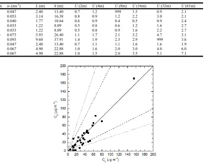
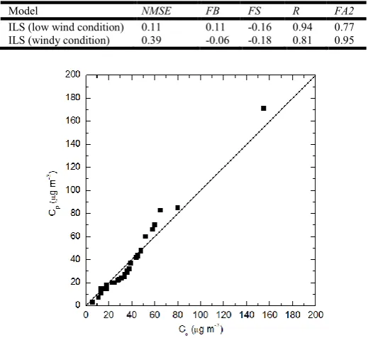
c _{is the Coriolis parameter.}

[image:5.595.103.509.442.765.2]

The model performances are shown in Table 2 and Figures 1 and 2. Table 2 shows the result of the statistical analysis made with observed and predicted values of ground-level centerline concentration. Figure 1 shows the scatter diagram between observed and predicted concentration. Figure 2 shows a quantile-quantile plot where the distribution of predicted and observed values are compared. In this figure the data are ordered by rank, so for instance the quantile of the predicted concentration is plotted against the same quantile of the observed concentration (Olesen, 1995). In this sense, this plot permits to compare the frequency distributions of predicted and observed data. The statistical indices are suggested by Hanna (1989):

Table 1. Meteorological data measured during the INEL experiment

run u*(ms-1) L (m) h (m) U (2m) U (4m) U (8m) U (16m) U (32m) U (61m)

4 0.047 2.40 13.40 0.7 1.2 999 1.5 0.9 2.1

5 0.053 3.14 16.38 0.8 0.9 1.2 2.2 3.0 2.1

7 0.040 1.77 10.64 0.6 0.9 0.4 0.5 0.9 2.4

8 0.033 1.22 8.09 0.5 0.8 0.6 1.2 1.6 2.7

9 0.033 1.22 8.09 0.5 0.8 0.9 1.6 2.2 2.7

10 0.073 5.93 26.40 1.1 1.7 2.1 3.2 4.7 3.1

11 0.093 9.60 37.91 1.4 1.9 2.3 2.9 999 3.6

12 0.047 2.40 13.40 0.7 1.1 1.1 1.6 1.6 1.9

13 0.067 4.90 22.88 1.0 1.6 2.0 3.0 4.0 6.0

14 0.067 4.90 22.88 1.0 1.5 2.0 3.5 5.1 7.1

Figure 1. Scatter diagram between observed (Co) and predicted (Cp) ground-level centerline concentration during INEL experiment.

[image:6.595.168.428.75.313.2]

Table 2. Statistical evaluation considering the model simulations for low wind and windy conditions

Model NMSE FB FS R FA2

ILS (low wind condition) 0.11 0.11 -0.16 0.94 0.77 ILS (windy condition) 0.39 -0.06 -0.18 0.81 0.95

[image:6.595.195.400.381.642.2]

Figure 2 - Model perfomance in terms of quantile-quantile considering low wind condition. Solid line indicates unbiased prediction

Table 3. Meteorological data measured during the Prairie Grass experiment

run L (m) h (m) µ*(ms-1) U (ms-1)

13 3.4 23 0.09 3.9

14 1.6 12 0.05 3.7

17 48 131 0.21 3.8

18 25 92 0.2 4

21 172 333 0.38 6.4

22 204 400 0.46 7.7

23 193 358 0.39 6.5

24 248 400 0.38 6.3

28 24 81 0.16 3.2

29 36 119 0.23 4.3

32 8.3 43 0.13 3.6

35 53 147 0.24 4.3

36 7.8 36 0.1 2.8

37 95 216 0.29 5

38 99 217 0.28 4.8

39 9.8 48 0.14 3.6

40 8 39 0.11 3.1

41 35 117 0.23 4.4

42 120 275 0.37 6.3

46 114 257 0.34 5.8

53 10 54 0.17 4.3

54 40 128 0.24 4.5

55 124 279 0.37 6.3

56 76 194 0.29 5.1

58 6.4 35 0.11 3.4

59 11 51 0.14 3.4

60 58 166 0.28 5

p o p

o

C

C

C

C

NMSE



(



)

2

/

(Normalized Mean Square Error)

))

(

5

.

0

/(

)

(

C

_o

C

_p

C

_o

C

_p

FB







(Fractional Bias)



o p

 

o p



FS



2













(Fractional Standard Deviation)

p o p p o

o

C

C

C

C

R



(



)(



)

/





(Correlation Coefficient)



2

[image:7.595.203.419.52.262.2]

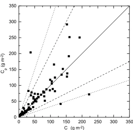
Figure 3 – Scatter diagram between observed (Co) and predicted (Cp) ground-level crosswind integrated concentrations for the Prairie

Grass experiment. Dashed lines indicate factor of 2, dotted lines indicated factor of 3 and solid line indicates unbiased prediction

Figure 4 - Model perfomance in terms of quantile-quantile considering windy condition. Solid line indicates unbiased prediction.

where

C

is the analyzed quantity (concentration) and the subscripts "o" and "p" represent the observed and the predicted values, respectively. The overbars in the statistical indices indicate averages. The statistical index FB indicates if the predicted quantity underestimates or overestimates the observed one. The statistical index NMSE represents the quadratic error of the predicted quantity in relation to the observed one. The statistical index FS indicates the measure of the comparison between predicted and observed plume spreading. The statistical index FA2 provides the fraction of data for which 0.5Co Cp2_{. As nearest zero are}

the NMSE, FB and FS and as nearest one are the R and FA2, better are the results. Giving a look at the results we promptly can observe that the ILS simulates quite well the experimental data when low wind occurs. The statistical analysis reveals that all indices are within acceptable ranges, with NMSE, FB and FS values are relatively near to zero and R and FA2 are relatively near to 1. It is important to say that these results are comparable or even better than ones obtained by other authors with different models (Sagendorf and Dickson, 1974; Sharan and Yadav, 1998; Oettl et al., 2001; Moreira et al., 2005). From the quantile-quantile analysis, it is possible to observe that the model behaviour is quite acceptable.

Windy Condition

Prairie Grass dispersion experiment was carried out in O'Neill, Nebraska, 1956. The tracer (SO2) was released without buoyancy

at a height of ~ 0.5 m and collected at a height of 1.5 m at three downwind distances (50, 200 and 800 m). The Prairie Grass site was quite flat and much smooth with a roughness length of 0.6 cm. We present here the results for 27 stable runs, for which the condition h/L0 _{is satisfied. The micrometeorological parameters recorded during the dispersion experiments are summarized in}

Table 3, based on the paper of van Ulden (1978). The wind speed profile is parameterized following the similarity theory of Monin-Obukhov and OML model (Berkowicz et al., 1986). The model performance is shown in Tables 2 and Figure 3 and 4. Table 2 shows the result of the statistical analysis made with observed and predicted values of ground-level cross-wind-integrated concentration (Cy_{). Figure 3 shows the scatter diagram between observed and predicted} Cy.

0 50 100 150 200 250 300 350

0 50 100 150 200 250 300 350

C p

(

g m

-2)

C

o (g m

[image:7.595.207.416.311.507.2]

Figure 4 presents a quantile-quantile plot where the distribution of predicted and observed values are compared. Analysing the statistical indices in Tables 1 it is possible to notice that the model simulates quite well the observed concentrations, with NMSE, FB and FS values relatively near to zero and R and FA2 very close to 1. The quantile-quantile plot reveals that the model presents a tendency for underestimate the highest concentration values.

Conclusion

In this work a semi-analytical model is proposed to investigate the contaminant dispersion in stable conditions. The model is based on the solution of the Langevin equation throught the Method of Successive Approximations or Picard’s Iterative Method. The novelty in this work is the consideration of the Eulerian autocorrelation function suggested by Frenkiel (1953) and Murgatroyd (1969) in the development of the equations for the turbulent velocities. By considering this formulation, the model is able to simulate the dispersion in the SBL during low wind conditions or during higher wind speeds, depending of the parameter associated with the characteristic period of the horizontal oscillation due the meander (

m

). In this new approach, when

m



0

the dispersion in the SBL is under meandering effect, which occurs during low wind conditions. In this case, the model is written in terms of the Frenkiel (1953) and Murgatroyd (1969) autocorrelation function, which generates a negative lobe in the horizontal velocity components. When m0_{, the meandering effect is eliminated, and the application of the model is limited to highest wind}

situations (u_{2.0 ms}-1

). In this case, the model is written in terms of the exponential form of the autocorrelation function (_etl

), in which the Lagrangian particle models usually make use when windy conditions are present. Therefore, low wind conditions are completely different from the more general case of moderate and strong winds (Anfossi et al., 2005). In this sense, the ILS technique is here suggested for the appropriate treatment of the pollutant dispersion in both conditions. Giving a closer look to the results reported in Tables 2 and Figures 1 - 4, we promptly realize that the ILS model gives good results. In the particular case of light wind stable conditions, the model results are better than ones obtained in other works. The statistical analysis reveals that all values for the indices are within ranges that are characteristics of those found for other state-of-the-art models applied to other field datasets. The quantile-quantile analysis show good results, mainly for the dispersion simulation during low wind conditions.

Acknowledgements

This work is partially supported by CNPq. (Conselho Nacional de Desenvolvimento Científico e Tecnológico) and FAPERGS (Fundação de Amparo à Pesquisa do Estado do Rio Grande do Sul).

REFERENCES

Anfossi, D., Oettl, D., Degrazia, G.A. and Goulart, A. 2005. An analysis of sonic anemomenter observations in low Wind speed conditions. Bound.-Layer Meteor. 1, 114, 179-203.

Barad M.L. 1958. Project Prairie Grass: A Field program in diffusion, Geophys. Res. Paper No 59 (II) TR-58-235 (II), Air Force Cambridge Research Centre, USA.

Berkowicz R.R., Olesen H.R. and Torp U. 1986. The Danish Gaussian air pollution model (OML): Description, test and sensitivity analysis in view of regulatory applications, Air Pollution Modeling and Its Application, C. De Wispeleare, F.A. Schiermeirier and N.V. Gillani Eds., Plenum Publishing Corporation, 453-480.

Boyce, W. and Di Prima, R. 2001. Elementary Differential Equations and Boundary Value Problems. John Wiley & Sons, Inc., 749 pp.

Brusasca, G., Tinarelli, G. and Anfossi, D. 1992. Particle model simulation of diffusion in low wind speed stable conditions. Atmos. Environ. 26A, 707-723.

Carvalho, J. C., Vilhena, M. T. and Moreira, D.M. 2005b. An alternative numerical approach to solve the Langevin equation applied to air pollution dispersion. Water Air and Soil Pollution. 163, 1-4, 103-118

Carvalho, J. C., Vilhena, M. T., Degrazia, G. A. and Sallet, M. 2013. A General Lagrangian Approach to Simulate Pollutant Dispersion in Atmosphere for Low-wind Condition. American Journal of Environmental Engineering, 3, 8-12.

Carvalho, J.C., Nichimura, E.R., Vilhena, M.T.M.B., Moreira, D.M. and Degrazia, G.A. 2005a. An iterative langevin solution of contaminant dispersion simulation using the Gram-Charlier PDF, Environmental Modelling and Software 20, 3, 285-289. Degrazia G.A., Anfossi D., Carvalho J.C., Mangia C., Tirabassi T. and Campos Velho H.F. 2000. Turbulence parameterization

for PBL dispersion models in all stability conditions. Atmos. Environ. 34 3575-3583.

Degrazia, G.A., Moraes, O.L.L. and Oliveira, A.P. 1996. An Analytical method to evaluate mixing length scales for the planetary boundary layer. Journal of Appl. Meteor. 35, 974-977.

Frenkiel, F.N. 1953. Turbulent diffusion: Mean concentration distribution in a flow field of homogeneous turbulence. Adv. Appl. Mech. 3, 61-107.

Hanna, S.R. 1989. Confidence limit for air quality models as estimated by bootstrap and jacknife resampling methods. Atmos. Environm. 23, 1385-1395.

Innocentini, V. 1999. A successive method for the evaluation of trajectories approximating the parcel by a linear function of space and time. Monthly Weather Review 127, 1639-1650.

Luhar A.K. and Britter R.E. 1989. A random walk model for dispersion in inhomogeneous turbulence in a convective boundary layer. Atmos. Environ. 23, 1191-1924.

Murgatroyd, R.J. 1969. Estimations from geostrophic trajectories of horizontal diffusivity in the mid-latitude troposphere and lower stratosphere. Quart. J. Roy. Meteorol Soc. 95, 40-62.

Oettl, D. and Anfossi, D. 2005. Personal Communication.

Oettl, D., Almbauer, R.A. and Sturm, P.J. 2001 A new method to estimate diffusion in stable, low-wind conditions. J. Appl. Meteor. 40, 259-268.

Olesen, H.R. 1995. Data set and protocol for model validation. Workshop on Operational Short-Range Atmospheric Dispersion Models for Environmental Impact Assessment in Europe, Mol, Belgium. Int. J. Environm. and Pollution 5, 4-6, 693-701. Sagendorf, J.F. and Dickson, C.R. 1974. Diffusion under low wind-speed, inversion conditions, U.S. National Oceanic and

Atmospheric Administration Tech. Memorandum ERL ARL-52.

Shankar Rao, K. 1999. Lagrangian Stochastic Modeling of Dispersion in the Stable Boundary Layer, 90, 3, 541-549.

Sharan, M. and Gopalakrishnan, S.G. 2003. Mathematical modeling of diffusion and transport of pollutants in the atmospheric boundary layer. PAGEOPH, 160, 357-394.

Sharan, M. and Yadav, A.K. 1998. Simulation of experiments under light wind, stable conditions by a variable K-theory model. Atmos. Environ. 32, 3481-3492.

Van Ulden A.P. 1978. Simple estimates for vertical dispersion from sources near the ground, Atmos. Environ., 12, 2125-2129. Weil, J.C., Sullivan, P.P. and Moeng, C.H. 2004. The use of Large-eddy simulation in Lagrangian particle dispersion models, J.

Atmos. Sci., 61, 2877-2887.

Zannetti, P. 1990. Air Pollution Modelling. Computational Mechanics Publications. Southampton. 444pp.

Zilitinkevith, S.S. 1972. On the determination of the height of the Ekman boundary layer. Boundary-Layer Met. 3, 141-145.