Investigating the Process of Exporting Autodesk Ecotect
Models to Detailed Thermal Simulation Software
Tamer Gado
1, Mady Mohamed
2,*1Dundee School of Architecture, University of Dundee, UK
2Zagazig Department of Architecture, Zagazig University, Egypt
*Corresponding Author: [email protected]
Copyright © 2014Horizon Research Publishing All rights reserved
Abstract
Autodesk Ecotect 1 is a whole buildingsimulation software that can predict the thermal, visual and acoustic performance of buildings. It is very user-friendly software that could potentially integrate with the architectural design process. Thermal performance analysis in Autodesk Ecotect is based on the Chartered Institution of Building Services Engineers (CIBSE) admittance method and thus inherits its limitations. Hence, the need to use more detailed thermal simulation tools during the final stage of a building design or research project. This paper investigated the potential of using detailed thermal simulation software (HTB2) in conjunction with Autodesk Ecotect. Five primary classrooms built in a hot-dry climatic region were monitored. The same classrooms were modelled in Autodesk Ecotect using several modelling techniques and the internal temperatures were simulated using HTB2. Analysis of results suggested that a number of necessary measures are required to ensure the reliability and accuracy of the simulation results.
Keywords
Thermal Simulation, Autodesk Ecotect Models, Primary Schools, Hot-Dry Climate, Building Thermal Performance, Computer Modelling1. Research Background and Previous
Work
Computer modelling can allow architecture practitioners, researchers and students to predict the energy efficiency and environmental behaviour of buildings. There are a wide range of detailed thermal simulation software available such as HTB22, DEROB-LTH3, DOE-2, EnergyPlus4 and ESP-r5.
1 At the time of writing up this paper, Ecotect was own by Sqaure One
Research Ltd. Late June 2008, Autodesk had aquired Ecotect and the later is now known as Autodesk Ecotect <http://usa.autodesk.com/adsk/servlet/ind ex?id=11778740&siteID=123112>.
2 http://www.cardiff.ac.uk/archi/ComputerModelling.php 3 http://www.derob.se
4 http://www.eere.energy.gov/buildings/energyplus 5 http://www.esru.strath.ac.uk/Programs/ESP-r.htm
The interfaces of those packages are complicated and they require a fair amount of experience in computer modelling. In addition, they all need substantial time to master. This limits the integration of simulation within the architectural design process. It is relatively difficult to input building geometry to these software tools as well as to interpolate the simulation results. The model has to be introduced in some cases in textual format. This - sometimes - leads to inaccuracy due to human error during data input, consumes time and requires advanced knowledge of computer programming. This also does not fit with the mode of thinking in architectural practice and education.
More architects need to quickly and easily check the environmental impact of their designs in order to reduce carbon dioxide emissions and conserve energy and to comply with legislation. Whole building simulation 3D based programmes such as IES6, Autodesk Ecotect7 can
allow the three dimensional visualization of the unseen environmental attributes of architectural spaces. This can facilitate more effective understanding of the issues involved in the quantification of the environmental performance of buildings. Geometric data are introduced to those tools either from CAD programs or directly using their 3D-based interfaces. Flexibility and ease of building 3D models varies from one tool to another.
Autodesk Ecotect has one of the most user-friendly interfaces that allows easy construction and manipulation of 3D models. User can import 3D computer models in *.3ds or *.dxf formats from several widely used computer aided design software such as AutoCAD, 3D Studio, Rhinoceros or Sketchup. Autodesk Ecotect version 5.6 is able to import and export gbXML. This facilitates more flexible communication with ArchiCAD and several other simulation and modelling tools [10]. From experience Autodesk Ecotect’s thermal simulation results are not fully representative of reality, although this is perhaps not an issue in case of parametric studies investigating the relative effectiveness of design options.
6 http://www.iesve.com 7 http://www.ecotect.com
This is the main disadvantage of Autodesk Ecotect. This is due to the limitations of its thermal simulation engine which is based on the CIBSE Admittance Method [4]. Autodesk Ecotect uses this method to calculate internal temperatures and heat loads. Admittance Method is a pseudo-dynamic method based on variation about the mean value. It also has the disadvantage of not taking in consideration the effect of solar radiation when it enters the space. Solar radiation is considered a space load the moment it hits a window and is not traced to check which internal surface it hits and accordingly heats up. Equally important Autodesk Ecotect cannot calculate thermal lag for composite elements that are not included in its library. Although the Autodesk Ecotect materials library includes most of the typical components used in the building industry, it does not cover a wide range of materials used throughout the world, especially outside Western countries. This prevents the user from optimizing the construction of his proposed design and therefore inhibits one of the main aims of computer simulation. Thus it is advised to use more detailed thermal simulation tools in later stages of design process or research projects.
Autodesk Ecotect model can be exported to a wide range of well established detailed thermal modelling software such as ESP-r, EnergyPlus, DOE-2 and HTB2. The following is a brief discussion of the advantages and disadvantages of those tools.
ESP-r was developed at the Energy Systems Research Unit of the University of Strathclyde. It simulates the thermal, visual and acoustic performance of buildings. It can also be used to assess the energy use and run computer fluid dynamics (CFD) analysis. Its thermal simulation engine uses a finite volume conservation method. ESP-r was subjected to a substantial number of validation studies including inter-model comparisons and comparisons with monitored data [11]. ESP-r is designed for UNIX operating system but can run under Cygwin environment. This still requires an advanced level of proficiency in UNIX. Despite its graphical user interface, it is still very user unfriendly for architects and architecture students. It is thus unlikely to be used during architectural design.
EnergyPlus was developed by the U.S Department of Energy. It models heating, cooling, lighting, ventilating loads. It is based on DOE-2.1 and BLAST features. It reads input and writes outputs as text files with a very unfriendly user interface. Lately several interfaces were developed including OpenStudio. This is a free plugin for Google SktchUp; a 3D modelling software widely used in architecture practices and schools. The main limitation of Energy Plus is that it does not accept more than four sided thermal zones. Although this is not a prohibitive problem in the majority of cases, it is impossible to use Energy Plus to study non-rectangular shapes or non-traditional designs.
HTB2 is a general purpose dynamic energy and environmental performance simulation tool. It is based on a simple Finite Difference Heat transport model [7] and can calculate internal temperature and energy use. It is “an example of a Detailed Simulation Programme or DSP. As
such it is complex software and can require a considerable learning effort to achieve its full potential” [1]. It generates its own heat flow coefficients and response factors from the detailed information of the layers making up composite building materials. This overcomes Autodesk Ecotect’s inability to calculate thermal time lag of composite materials. The main disadvantages of HTB2 are its inability to handle complex occupancy profiles and its inability to handle complex glazing and shading systems. In Previous work, Alexander et al [2] looked into developing HTB2 algorithms to be able to handle calculating the effect of glazing and shading options such as slatted blinds. They modified the algorithm to be capable of predicting total solar transmission of glazing with mid-pane shading combinations.
HTB2 can be linked to several software tools such as Autodesk Ecotect and the air-conditioning system simulation program BECON. The later could be used in conjunction with HTB2 to assess the electricity consumption for air-conditioning systems. This was used for example by Yik et al (YIK F. W. H., JONES P., & J., 2008) to assess the electricity consumption for air-conditioning in high-rise buildings in Hong Kong.
No previous work was found to investigate the research problem that the current paper is trying to address; “using Autodesk Ecotect and HTB2 as modelling and simulation tools simultaneously”. Only Marsh and Al-Oraier [8] employed Autodesk Ecotect in a previous work to build a model of a traditional adobe dwelling and exported it to HTB2 and Energy plus. They studied the issues associated with creating a base computer model in Autodesk Ecotect that is fully compatible with HTB2 and EnergyPlus simulation tools. They then compared the two outputs to the monitored data. They found reasonably close agreement between the simulated and monitored data. However, in some cases they found significant variation between the results of the two software tools and the measured data and between the results of the two software tools themselves. This close agreement between the simulated results and the measured data was unsupported quantitatively. Moreover, this work did not discuss the methods and constrains associated with exporting the model from Autodesk Ecotect to HTB2.
2. Research Aims
specification and weather data, 2) the method by which the Autodesk Ecotect model is introduced to HTB2. The later is the focus of the work presented in this paper. Being able to easily and quickly present the situation in question and yet generate reliable representation of real situations is an important factor in any simulation study. This work investigated the model setting and geometry to build a base computer model in Autodesk Ecotect that could be exported and simulated in HTB2 properly. Graphical and statistical tests will be employed to quantify the strength of the closeness between both the monitored and simulated sets of data.
3. Methodology and Research Climatic
Context
This work considers rules and procedures for importing Autodesk Ecotect models to the detailed thermal simulation software HTB2.
[image:3.595.325.535.167.647.2]Geometric and physical descriptions of the five classrooms are modelled in Autodesk Ecotect and their performance simulated. The depth and complexity of the models are varied. The simulation output is then compared to measured data for the month of May.
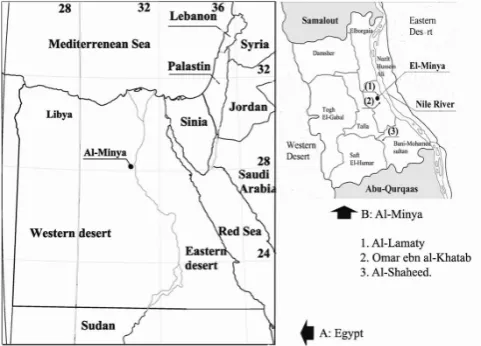
Figure 1. a) Map of Egypt with the location of al-Minya and Belbas, b) Skem school location in Beblas, c) Case studies location in al Minya: 1- al-Lamaty 2 – Omar ebn al-Khatab 3- al-Shaheed
To this end, five classrooms of three governmental primary schools built in al-Minya Governorate of the Arab Republic of Egypt (refer to Figure 1) were employed as a vehicle for the investigation these are a) Omer ebn al-Khatab school, b)Al-Lamaty school and c) Al-Shaheed school.
Egypt is situated in the northeast corner of Africa (27 00N and 30 00E). According to Köppen-Geiger climate classification system, Egypt lies in the warm desert climatic zone [12]. The country is further divided into seven climatic design regions. Al-Minya lies in the desert climatic design
zone. This zone is the largest among the seven regions. It is characterised by large diurnal variation with typical average outdoor day air temperatures of 41oC and typical night
average air temperature of 20.5oC in August, and typical
average low outdoor air temperature of 4 oC in winter.
The three schools employed vary in size; form and orientation as shown in Figure 2
a)
b)
c)
Figure 2. a) Omar ebn al-khatab, b) Al-Lamaty, c) Al-Shaheed
[image:3.595.58.299.381.554.2]Figure 3. Typical plan and section of the governmental primary schools built by GAEB including the location of the temperature and humidity data loggers and sensors
[image:4.595.93.521.557.722.2]The internal air temperatures inside all the classrooms were monitored during May 2007; the hottest month of the academic year. This was done using Hobo U12 data loggers. Outdoor temperature ranged between 43.42 oC and 15.62 oC.
Relative humidity ranged between 72.25% and 6.75%. External weather data during the same period were logged using a Hobo weather station to create a weather file that was used later in the thermal simulation.
The effect of 13 modelling and exporting conventions and rules provided by Autodesk Ecotect developer [9, 10] on the effectiveness of communicating with HTB2 and the reliability of the simulation results, were investigated. Those conventions can be summarised as:
Each zone must be drawn as an enclosed three dimensional prism with planar surfaces on all sides. In other words, each zone must be ‘air tight’ volume. Autodesk Ecotect will only consider a volume of space as a thermal zone if its surfaces fully enclose the entire volume;
Two zones are considered to be adjacent if they are parallel to each other and less than a specified distance apart known as adjacency tolerance. This must be adjusted to accommodate the separation distance as appropriate depending on the modelling technique applied;
All the types of elements and materials used have to be specified;
Each space of the building under investigation must be drawn as a separate zone;
If a space is adjacent to or includes another secondary space that exchange air with, then the secondary space could be added to the primary zone;
A large open-plan space with windows in several sides must be divided into several sub-zones;
The shared elements between two adjacent zones must be adjacent and overlapping;
External shading systems must be placed on a non-thermal zone so as not to contribute to the thermal zone;
In order for Autodesk Ecotect to recognize the orientation of each surface, especially in very complex models, the normals of all the surfaces must point outwards [9, 10].
Further three modelling inputs were varied; the model size, voids construction and wall construction detailing.
Omer ebn al-Khatab classroom was modelled. Upon exporting the Autodesk Ecotect model to HTB2, an error occurred. Two reasons were found; the method of void construction and the model size (refer to sections 4.1 and 4.2). Upon resolving these issues the Autodesk Ecotect model was successfully exported to HTB2. Simulated internal air temperatures were compared to the monitored internal air temperatures graphically (Figure 9) and statistically using Mann-Whitney test. A significant difference (p<0.05) was found. A parametric analysis was conducted and it was found that the level of model details has a statistically significant effect on the reliability of the simulation results. The level of details that yielded internal air temperatures closest to the
monitored data was further used.
To investigate the collective effect of all rules and particularly the effect of the proposed level of details, the other four classrooms were modelled using all rules listed. Once again the internal air temperatures of the classrooms were simulated using HTB2 and the results were compared statistically to the monitored data. Applying Mann-Whitney test on the simulated and the monitored temperatures suggested that the difference in all cases was not significant (p>0.05).
4. Modelling Conventions and Rules
4.1. Modelling for Autodesk Ecotect simulation
There are several methods of building a 3D model in Autodesk Ecotect. The choice depends mainly on the stage of the design process. The straight forward method is to build the model directly on Autodesk Ecotect. An alternative way is to import the 3D model from other software such as Sketchup, AutoCAD or Rhinoceros in DXF or 3ds format. This method will result in a very large file, which will affect the simulation speed. In other cases, exporting the 3D model from other software might result in a complex Autodesk Ecotect model, which will not be suitable for running thermal simulation. In case of lighting analysis, the user might want to model the building in detail if this is expected to affect the simulation results. Another technique is to trace over a scanned hand drawn or computer sketch using either the centre line of the walls or the internal boundaries of each space to build the thermal zones. This method is expected to be very popular in architectural context as it allows checking a wide range of options very early on during the design process.
If a model is drawn in Autodesk Ecotect properly, the thermal simulation will run smoothly. However, not every Autodesk Ecotect model will successfully be exported to and simulated by HTB2.
4.2. Modelling for Exporting to HTB2
There are several sets of limitations that must be adhered to during Autodesk Ecotect model construction to successfully communicate with HTB2. According to Autodesk Ecotect documentation [6] there are three main rules:
shown in Figure 5;
Figure 5. Replacing several windows on the same wall with a single window of the same combined area
In addition, HTB2 documentation adds the following limitations:
100 modelled and 3 un-modelled spaces;
25 construction types, using a total of 100 parts;
25 window types and 100 shading masks;
600 elements, with 9000 fabric nodes; 100 heating systems.
2. Each window must be assigned to the object onto which any direct solar radiation will fall. By default Autodesk Ecotect assigns this to the floor of the zone in which the window is located. If Autodesk Ecotect is unable to find an associated floor object, it will choose another zone object and generate a warning message; 3. HTB2 does not use the thermal properties of
composite elements that Autodesk Ecotect generates. Instead it generates its own heat flow coefficients and response factors from the detailed layers information. If the properties of any layer used to build up a material in Autodesk Ecotect are not accurate or not specified, HTB2 will generate an error message and the exporting process will be aborted;
5. Convention and Rules Application
One case study - Omar ebn al-Khatab – was modelled in Autodesk Ecotect taking in consideration all previously mentioned conventions. On exporting the model to HTB2, numerous error messages were displayed and the exporting process was stopped. The error messages in most cases did not provide enough guidance on how to fix the faults in the model. For example, when an Autodesk Ecotect model including a curved surface drawn as an arch was exported to HTB2, the process was stopped, and the following error message was displayed: ERROR: RDLAY: inappropriatesurface area has been specified. It was not clear from this
message which surface caused the error and why it was inappropriate. Accordingly a parametric analysis was conducted to pinpoint the cause of error. Two reasons were found: 1) model size, 2) the method of voids construction and modelling technique developed that overcame these errors.
5.1. Model Size
In some cases, it is difficult not to exceed the limitations on the number of model elements especially the restriction on total number of elements of the model (refer to point 4 under section 3.2). The model of any multi-storey building could easily exceed this limit if built to a reasonable level of details. The current work proposes several recommendations to reduce the total number of elements while maintaining a fair level of reliability. Those recommendations could be summarised as follows:
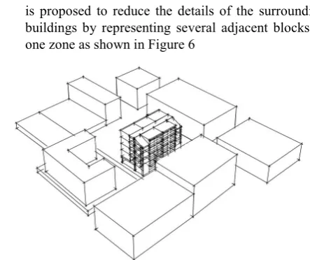
1. Itis important to include the overshadowing effect due to surrounding buildings. However, modelling the surrounding buildings could substantially increase the total number of elements in the model. To avoid this it is proposed to reduce the details of the surrounding buildings by representing several adjacent blocks as one zone as shown in Figure 6
Figure 6. Surrounding buildings drawn in Autodesk Ecotect as single non-thermal zones
[image:6.595.66.287.77.191.2]2. Reduce the details of the adjacent zones by using larger non-thermal zones as shown in Figure 7. “Autodesk Ecotect v5.50 will make any surface that is adjacent to one or more planar objects on a non-thermal zone into an adiabatic surface i.e. has no heat flow through it” [5]. This is valid in the case of, for example, a terraced house or a multi-storey building. In these cases the heat flow from adjacent zones could be ignored assuming that the temperatures inside them will be roughly the same as the zone under investigation
Figure 7. Reducing the number of elements of a multi-storey building
[image:6.595.319.541.231.417.2] [image:6.595.319.550.593.709.2]become of no use after completing the model and unnecessarily double the number of partitions in the model. Therefore, it is advised to delete those lines before exporting the model to HTB2.
5.2. Voids Construction
In two of the case studies, the classrooms are arranged on a linear single sided corridor exposed from one side to the elements as shown in Figure 3. One way of modelling this in Autodesk Ecotect is to construct a zone representing the
corridor and then insert a void in the external walls as shown in Figure 8a. HTB2 requires the detailed layer information of each object. Since void is not built up of layers, HTB2 could not handle it. Hence, an error message saying that there is an unknown source for the void layer was displayed when the model was exported from Autodesk Ecotect to HTB2. To overcome this problem it is proposed to delete the wall and build the solid parts around the void using a single plane as shown in Figure 8b. It is to be noted that this plane must be in the same zone and should be assigned a wall material..
[image:7.595.101.512.221.333.2]a. Void in a wall b. Solid part as a single Plane c. Solid parts as several partition
Figure 8. Techniques of building a void in Autodesk Ecotect
6. Results and Discussions
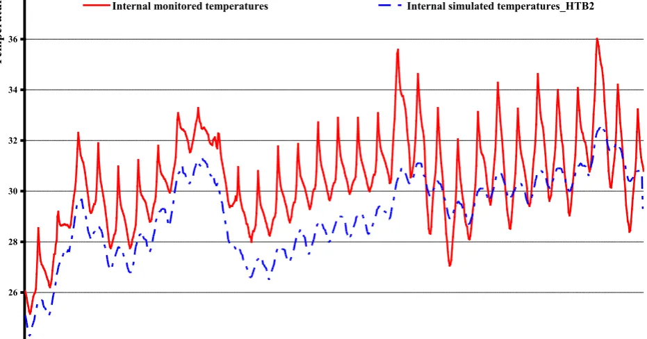
[image:7.595.73.539.446.690.2]Based on the above, the Autodesk Ecotect model was successfully exported to HTB2 and the thermal simulation was conducted. In order to validate the simulation results, the hourly simulated and monitored data were compared as shown Figure 9 .
Figure 9. The internal monitored air temperatures compared to the HTB2 simulated air temperatures
24 26 28 30 32 34 36 38
1 1 2 3 4 5 6 6 7 8 9 10 11 11 12 13 14 15 16 16 17 18 19 20 21 21 22 23 24 25 26 26 27 28 29 30 31 31
Days
T
em
pe
ra
tu
re
s
Applying Mann-Whitney test on the data revealed a significant difference (p<0.05), despite the two sets of data trends being consistent. One reason for this could be the fact that walls are constructed of different materials of different thicknesses as shown in Figure 10. Further work was conducted to investigate the effect of the model level of details on the accuracy of the simulation results.
Figure 10. Different materials used in the external wall, after Mohamed
7. Effect of Model Details on the
Simulation Accuracy
In order to investigate the effect the model level of details
on the simulation accuracy, a parametric analysis was conducted to optimize the level of details without jeopardizing the accuracy of the results. The first case study was modelled using the following four methods as follows: 1. All walls of all zones are drawn in full details. That is to say, every part of the wall is drawn as a single plain or partition and is specified a specific material; 2. Only walls of the zone under investigation are drawn
in full details with the rest of the building’s walls drawn in a simple manner. The later means, drawing the wall as a one element using the material properties of its largest section;
3. Only the zone under investigation is drawn in a simple form with the rest of the building drawn in full details; 4. All zones are drawn in simple form.
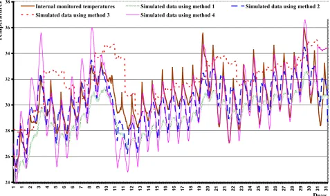
Figure 11 presents the HTB2 simulated internal air temperatures inside the classroom generated using the four modelling techniques. The simulated temperatures were then compared to the monitored data. Applying one way ANOVA test (F=205.39) on the data revealed that the mean internal air temperatures inside the four cases are significantly different (p<0.05). Applying Post Hoc LSD test on the data revealed that there is a significant difference (p<0.05) between the simulated internal air temperature and the monitored temperature in all cases except in case of using the second modelling technique.
Figure 11. Internal simulated air temperature generated using all wall modelling techniques compared to the monitored internal air temperature inside Omar ebn al-Khatab classroom.
24 26 28 30 32 34 36 38
1 1 2 3 4 5 6 6 7 8 9 10 11 11 12 13 14 15 16 16 17 18 19 20 21 21 22 23 24 25 26 26 27 28 29 30 31 31
Days
T
em
pe
ra
tu
re
s
Internal monitored temperatures Simulated data using method 1 Simulated data using method 2
[image:8.595.64.301.168.310.2] [image:8.595.70.548.409.692.2]8. Results Validation
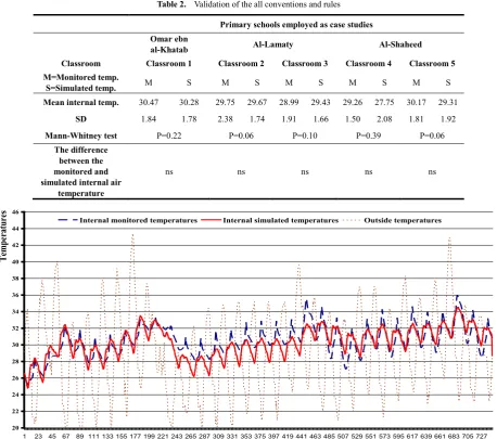
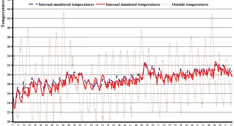
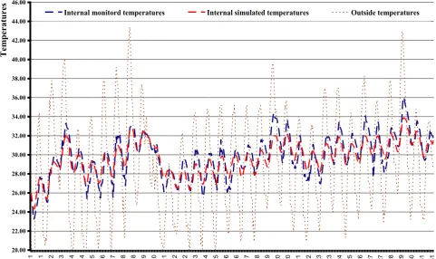
In order to validate the proposed conventions and rules in terms of the simulation results accuracy, the other four case studies were modelled using the technique that yielded internal temperatures closest to the monitored temperatures as described above. Models were then exported to HTB2 and the thermal simulation was performed. The simulation results were compared statistically to the monitored data using Mann-Whitney test. Analysis of results suggested that the difference between the simulated and the monitored temperatures in all cases is not significant (p>0.05) as shown in Table 2. Figures 12-16 graphically present a comparison between the simulated and monitored data inside the four case studies. They indicate a consistent trend of both sets of data.
Table 1. The effect of wall modelling techniques on the accuracy of the simulated internal air temperature
Internal air temperature
Monitored using method 1 Simulated Simulated using method 2 Simulated using method 3 Simulated using method 4
Mean 30.47 29.10 30.28 31.98 30.25
SD 1.84 1.64 1.78 1.78 2.57
ANOVA F=205.389, P=0.005 Significant
Table 2. Validation of the all conventions and rules
Primary schools employed as case studies Omar ebn
al-Khatab Al-Lamaty Al-Shaheed
Classroom Classroom 1 Classroom 2 Classroom 3 Classroom 4 Classroom 5
M=Monitored temp.
S=Simulated temp. M S M S M S M S M S
Mean internal temp. 30.47 30.28 29.75 29.67 28.99 29.43 29.26 27.75 30.17 29.31
SD 1.84 1.78 2.38 1.74 1.91 1.66 1.50 2.08 1.81 1.92
Mann-Whitney test P=0.22 P=0.06 P=0.10 P=0.39 P=0.06
The difference between the monitored and simulated internal air
temperature
ns ns ns ns ns
Figure 12. Internal simulated air temperature generated using the proposed wall modelling technique compared to the monitored internal air temperature inside Omar ebn al-Khatab (Classroom 1).
20 22 24 26 28 30 32 34 36 38 40 42 44 46
1 23 45 67 89 111 133 155 177 199 221 243 265 287 309 331 353 375 397 419 441 463 485 507 529 551 573 595 617 639 661 683 705 727
Hours/May
Te
m
pe
ra
tu
re
s
[image:9.595.101.510.206.299.2] [image:9.595.75.534.308.713.2]
Figure 13. Internal simulated air temperature generated using the proposed wall modelling technique compared to the monitored internal air temperature inside al-Shaheed School (Classroom 2).
Figure 14. Internal simulated air temperature generated using the proposed wall modelling technique compared to the monitored internal air temperature inside al-Shaheed School (Classroom 3).
20 22 24 26 28 30 32 34 36 38 40 42 44 46
1 1 2 3 4 4 5 6 7 8 8 9 10 11 12 12 13 14 15 16 16 17 18 19 20 20 21 22 23 23 24 25 26 27 27 28 29 30 31 31
Hours/May
T
em
pe
ra
tu
re
s
Internal monitored temperatures Internal simulated temperatures Outside temperatures
20 22 24 26 28 30 32 34 36 38 40 42 44 46
1 1 2 3 4 4 5 6 7 8 8 9 10 11 12 12 13 14 15 16 16 17 18 19 20 20 21 22 23 23 24 25 26 27 27 28 29 30 31 31
Hours/May
T
em
pe
ra
tu
re
s
[image:10.595.69.548.76.356.2] [image:10.595.65.546.403.661.2]Figure 15. Internal simulated air temperature generated using the proposed wall modelling technique compared to the monitored internal air temperature inside al-Lamaty School (Classroom 4).
Figure 16. Internal simulated air temperature generated using the proposed wall modelling technique compared to the monitored internal air temperature inside al-Lamaty School (Classroom 5).
20 22 24 26 28 30 32 34 36 38 40 42 44 46
1 1 2 3 4 4 5 6 7 8 8 9 10 11 12 12 13 14 15 16 16 17 18 19 20 20 21 22 23 23 24 25 26 27 27 28 29 30 31 31
Days
T
em
pe
ra
tu
re
s
Internal monitord temperatures Internal simulated temperatures Outside temperatures
20.00 22.00 24.00 26.00 28.00 30.00 32.00 34.00 36.00 38.00 40.00 42.00 44.00 46.00
1 1 2 3 4 4 5 6 7 8 8 9 10 11 12 12 13 14 15 16 16 17 18 19 20 20 21 22 23 23 24 25 26 27 27 28 29 30 31 31
Days
T
em
pe
ra
tu
re
s
[image:11.595.66.548.419.705.2]9. Further Work
During the course of this work, four main gaps in the knowledge were identified that further work will address. These are:
1. The effect of weather files type (on-site monitored weather data, typical metrological year or synthesized) on the accuracy of the thermal simulation;
2. The generation of weather file from outdoor data logged on site;
3. The effect of modelling techniques and computer processing powers on the duration of simulation; 4. The effect of the simulation engine (admittance
method verses Finite Difference Heat transport model) on the simulation accuracy.
REFERENCES
[1] Alexander, D. K. (1996). HTB2 User Manual: A model for
the thermal environment of building in operation. Cardiff: Welsh School of Architecture, University of Wales College of Cardiff.
[2] Alexander, D. K., Hassan, K. A. K. & Jones, P. J. (1997)
Simulation of solar gains through external shading devices. IBPSA Conference. Prague, Czech Republic The International Building Performance Simulation Association, .
[3] Alexander, D. K.., Mylona, A. & Jones, P. J. (2005) The
simulation of glazing systems in the dynamic thermal model HTB2 Ninth International IBPSA Conference. Montréal,
Canada.
[4] CIBSE. (1999). Environmental design, CIBSE Guide A.
London: Yale Press Ltd.
[5] AUTODESK ECOTECT. (2013a). Autodesk Ecotect v5 Help:
Adiabatic Surfaces – Objects Adjacent tp Non-Thermal Zones (Version 5.5) [Comprehensive environmental analysis tool]: Square One research.
[6] AUTODESK ECOTECT. (2013b). Autodesk Ecotect v5
Help: Exporting to HTB2 (Version 5.5) [Comprehensive environmental analysis tool]: Square One research.
[7] AUTODESK ECOTECT. (2013c). Autodesk Ecotect v5 Help:
Thermal analysis (Version 5.5) [Comprehensive environmental analysis tool]: Square One research.
[8] Marsh, A. & Al-Oraier, F(2005) A comparative analysis
using multiple thermal analysis tools. International Conference “Passive and Low Energy Cooling for the Built Environment. Santorini, Greece.
[9] Marsh, A. J. (2006). Thermal Modelling: The AUTODESK
ECOTECT Way. Natural frequency July 04(002).
[10] Marsh, A. J. (2013). Autodesk Ecotect 2011 new features.
[11] Strachan, P. (2000). ESP-r: Summary of validation studies
(Technical report). Glasgow: Energy Systems Research Unit, University of Strathclyde.
[12] Peel, M. C., Finlayson, B. L., & McMahon, T. A. (2007).