Comparative Study of Artificial Neural Network and
Response Surface Methodology for Modelling and
Optimization the Adsorption Capacity of Fluoride onto
Apatitic Tricalcium Phosphate
M.Mourabet
*, A. El Rhilassi, M.Bennani-Ziatni, A. Taitai
Team Chemistry and Valorization of Inorganic Phosphates, Department of Chemistry, Faculty of Sciences, BP 133, Kenitra, Morocco *Corresponding Author: [email protected]
Copyright © 2014 Horizon Research Publishing All rights reserved.
Abstract
In this study, Response Surface Methodology(RSM) and Artificial Neural Network (ANN) were employed to develop an approach for the evaluation of fluoride adsorption process. A batch adsorption process was performed using apatitic tricalcium phosphate an adsorbent, to remove fluoride ions from aqueous solutions. The effects of process variables which are pH, adsorbent mass, initial concentration, and temperature, on the adsorption capacity ( 𝓆𝓆ℯ (mg/g)) of fluoride were investigated through three-levels, four-factors Box-Behnken (BBD) designs. Same design was also utilized to obtain a training set for ANN. The results of two methodologies were compared for their predictive capabilities in terms of the coefficient of determination(𝑅𝑅2), root mean square error (𝑅𝑅𝑅𝑅𝑅𝑅𝑅𝑅), and the absolute average deviation (𝐴𝐴𝐴𝐴𝐴𝐴) based on the experimental data set. The results showed that the ANN model is much more accurate in prediction as compared to BBD.
Keywords
Response Surface Methodology,Box-Behnken Designs, Artificial Neural Network, Adsorption Capacity, Fluoride
1. Introduction
Response Surface methodology (RSM), introduced by Box and Willson [1], is a collection of mathematical and statistical technique useful for analyzing problems in which several independent variables influence a dependent variable or response and the goal is to optimize the response[2]. The design procedure of response surface methodology is as follows [3]:
1. Designing of a series of experiments for adequate and reliable measurement of the response of interest.
2. Developing a mathematical model of the second order response surface with the best fittings.
3. Finding the optimal set of experimental variables that produce a maximum or minimum value of response. 4. Representing the direct and interactive effects of
process variables through two and three dimensional plots.
A second-order (quadratic) model is commonly used in response surface methodology:
𝒴𝒴 = 𝛽𝛽0+ ∑𝓀𝓀𝒾𝒾=1𝛽𝛽𝑖𝑖𝑥𝑥𝒾𝒾+ ∑𝒾𝒾=1𝓀𝓀 𝛽𝛽𝒾𝒾𝒾𝒾𝑥𝑥𝒾𝒾2+ ∑𝒾𝒾=1𝓀𝓀−1∑𝓀𝓀𝒾𝒾=𝒾𝒾+1𝛽𝛽𝒾𝒾𝒾𝒾𝑥𝑥𝒾𝒾𝑥𝑥𝒾𝒾+ ℰ (1) where 𝒴𝒴 is the process response or output (dependent variable); 𝑥𝑥1 , 𝑥𝑥2, … , 𝑥𝑥𝓀𝓀 are the input factors; 𝛽𝛽0 , 𝛽𝛽𝒾𝒾𝒾𝒾 (𝒾𝒾 = 1,2,…,𝓀𝓀) , 𝛽𝛽𝒾𝒾𝒾𝒾 (𝒾𝒾 = 1,2, … , 𝓀𝓀; 𝒾𝒾 = 1,2, … , 𝓀𝓀) are unknown parameters and ℰ is a random experimental error term assumed to have a zero mean.
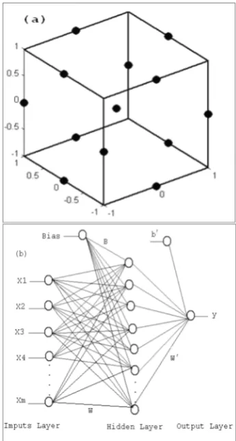
The most common second-order RSM designs are Box-Behnken (BBD) design and the Central Composite Design (CCD) with its variants. Box–Behnken design is a three-level design based on the construction of a balanced incomplete block design [4]. The BBD is an efficient option for fitting response surfaces using three evenly spaced levels [5]. Fig.1 (a) illustrates a Box-Behnken design for three factors. The number of experimental points (𝒩𝒩) is defined by the expression 𝒩𝒩 = 2𝓀𝓀(𝓀𝓀 − 1) + 𝒸𝒸𝑝𝑝 , where 𝓀𝓀 is the number of variables and 𝒸𝒸𝑝𝑝 is the number of center points [5].
output layer. The number of input and output neurons is fixed by the nature of the problem.
[image:2.595.92.265.251.573.2]The objective of a neural network is to compute output values from input values by some internal calculation [7]. Among the various types of neural networks, the feed-forward network with back propagation algorithm is the most widely used in different applications [8-13]. In the feed-forward ANN, the information is processed in the forward direction from input layer to hidden and then output layer obtained as the output of the network. The function of the hidden neurons is to intervene between the external input and the network response. The connection between inputs, hidden and output layers consist of weights and biases that are considered parameters of the neural network.
Figure 1. (a) Box-Behnken design for three factors. (b) Structure of a three-layer feed-forward network of 𝓂𝓂 inputs, hidden layer with 𝓀𝓀
neurons, output layer and 1 output.
For a three-layer feed-forward ANN (Fig.1 (b)), the ℓ𝑡𝑡ℎ estimated response, yℓ , that can be expressed:
𝒴𝒴ℓ = 𝜓𝜓
𝑜𝑜�𝑏𝑏′+ ∑𝓀𝓀𝒾𝒾=1𝑤𝑤𝒾𝒾′𝜓𝜓ℎ(∑𝒾𝒾=1𝓂𝓂 𝑤𝑤𝒾𝒾𝒾𝒾𝓍𝓍𝒾𝒾ℓ+ 𝑏𝑏𝒾𝒾)� (2) where,𝒲𝒲 = (𝑤𝑤𝒾𝒾𝒾𝒾) and ℬ = (𝑏𝑏𝒾𝒾) are the weight matrix and bias matrix of hidden layer, 𝒲𝒲′ = (𝑤𝑤
1′, 𝑤𝑤2′, … . , 𝑤𝑤𝓀𝓀′) and 𝑏𝑏′(scalar)are the weight matrix and bias of output layer,
𝑌𝑌 = (𝒴𝒴1, 𝒴𝒴2, … , 𝒴𝒴ℓ)′ is response vector, Χ
𝒾𝒾 is the ith input vector (𝛸𝛸𝒾𝒾= �𝓍𝓍𝒾𝒾1, 𝓍𝓍𝒾𝒾2, … , 𝓍𝓍𝒾𝒾ℓ′�′′′′
′′′
′; 𝒾𝒾 = 1,2, … , 𝓂𝓂) ,and 𝜓𝜓𝒽𝒽 , 𝜓𝜓𝑜𝑜 are transfer functions of hidden layer and output layer respectively.
Three types of commonly used transfer functions are as follows:
Linear transfer function
ψ(𝓍𝓍) = 𝓍𝓍 , −∞ < 𝜓𝜓(𝓍𝓍) < +∞ (3) Sigmoid transfer function
ψ(𝓍𝓍) =1+𝑒𝑒1−𝓍𝓍 , 0 ≤ ψ(𝓍𝓍) ≤ 1 (4)
Hyperbolic tangent transfer function
ψ(𝓍𝓍) =1+𝑒𝑒2−2𝓍𝓍− 1 , −1 ≤ ψ(𝓍𝓍) ≤ 1 (5)
Response surface methodology (RSM) and artificial neural network (ANN) methods are now successfully used jointly for both modeling and optimization purposes in many areas of science and engineering [13, 14-20]. In these studies, ANN and RSM techniques were compared for their predictive and generalization capabilities, sensitivity analysis and optimization abilities. It was found that the ANN model fit the data better and has higher predictive capability than RSM, even with the limited number of experiments.
However, there are only a few applications of ANN with RSM for the modeling of adsorption process [21-23]. Hence, the main motivation behind this study is the using the RSM and ANN methodologies for predicting the adsorption capacity of fluoride by apatitic tricalcium phosphate and the results which were obtained through RSM were then compared with those through ANN.
2. Material and Methods
2.1. Adsorbent
The apatitic tricalcium phosphate (Ca9 (HPO4)
(PO4)5(OH)) powders were prepared by an aqueous double
decomposition of the salts of calcium and of phosphate [24-25].
2.2. Batch Adsorption Experiments
2.3. Experimental Design
2.3.1. Response Surface Methodology
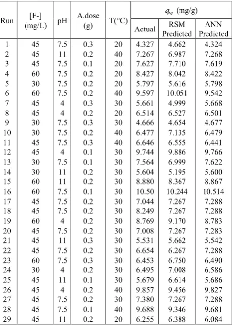
A three-level four factor Box-Behnken experimental design was generated with the Design- Expert 7.0.0 software. Initial concentration (30–60mg/L), pH (4–11), adsorbent dose (0.1–0.3g) and temperature (20–40°C) were input variables, the factor levels were coded as −1 (low), 0 (central point), and 1 (high). The design of real experiments is given in Table 1.
The response variable, 𝓆𝓆ℯ (adsorption capacity, mg/g) can be expressed as a function of the independent process variables (initial concentration(𝓍𝓍1), pH (𝓍𝓍2), adsorbent dose (𝓍𝓍3) and temperature (𝓍𝓍4)) according to the following response surface quadratic model:
𝓆𝓆ℯ = 𝛽𝛽0+ 𝛽𝛽1𝓍𝓍1+ 𝛽𝛽2𝓍𝓍2+ 𝛽𝛽3𝓍𝓍3+ 𝛽𝛽4𝓍𝓍4+ 𝛽𝛽11𝓍𝓍12+ 𝛽𝛽22𝓍𝓍22+ 𝛽𝛽33𝓍𝓍32+ 𝛽𝛽44𝓍𝓍24+ 𝛽𝛽12𝓍𝓍1𝓍𝓍2+ 𝛽𝛽13𝓍𝓍1𝓍𝓍3+ 𝛽𝛽14𝓍𝓍1𝓍𝓍4+ 𝛽𝛽23𝓍𝓍2𝓍𝓍3+ 𝛽𝛽24𝓍𝓍2𝓍𝓍4+ 𝛽𝛽34𝓍𝓍3𝓍𝓍4 (7) The coefficients, i.e. the model constant 𝛽𝛽0 , the linear terms (𝛽𝛽1, 𝛽𝛽2, 𝛽𝛽3, 𝛽𝛽4) , the quadratic terms (𝛽𝛽11, 𝛽𝛽22, 𝛽𝛽33, 𝛽𝛽44) , and the interaction terms (𝛽𝛽12, 𝛽𝛽13, 𝛽𝛽14, 𝛽𝛽23, 𝛽𝛽24, 𝛽𝛽34) , have been estimated from the experimental results applying least square method.
2.3.2. Artificial Neural Network
In this study, Neural Network Toolbox 8.0 of MATLAB mathematical software was used for simulation. The same experimental data, which had been used for the RSM design, were also employed in designing the artificial neural network. The input variables were initial concentration, pH, adsorbent dose and temperature. The corresponding adsorption capacity was used as a target.
The data were randomly divided into three groups, 70% in the training set, 15% in the validation set and 15% in the test set.
The tangent sigmoid transfer function (tansig) at hidden layer and a linear transfer function (purelin) at output layer were used. The similar transfer function was also used by Oguz and Ersol [26], Elmolla et al [27] and Khajeh et al [11].The training function selected for the network is ‘trainlm’. ’Trainlm’ is a network training function that updates weight and bias values according to the Lavenberg-Marquardt algorithm.
All variables and response were normalizedbetween 0 and 1 for the reduction of network error and higher homogeneous results. The normalization equation applied is as follows:
𝒴𝒴𝓃𝓃=𝒴𝒴𝓂𝓂𝒶𝒶𝓂𝓂𝒴𝒴𝒶𝒶−𝒴𝒴−𝒴𝒴𝓂𝓂𝒾𝒾𝓃𝓃𝓂𝓂𝒾𝒾𝓃𝓃 (8) where 𝒴𝒴𝓃𝓃 , 𝒴𝒴𝑎𝑎 , 𝒴𝒴𝓂𝓂𝒾𝒾𝓃𝓃 and 𝒴𝒴𝓂𝓂𝒶𝒶𝓂𝓂 are normalized value, actual value, minimum value, and maximum value, respectively.
3. Results and Discussion
3.1. Response Surface Methodology
Based on the experimental results of BBD in Table 1, a quadratic polynomial was established to identify the relationship between adsorption capacity and process variables. The resulting RSM model equation is following:
[image:3.595.315.552.407.739.2]𝓆𝓆ℯ= 8.8117 − 0.0406𝓍𝓍1− 0.3381𝓍𝓍2− 14.0445𝓍𝓍3+ 0.0582𝓍𝓍4+ 0.0012𝓍𝓍12− 0.0084𝓍𝓍22− 37.3792𝓍𝓍32+ 0.0018𝓍𝓍42+ 0.0048𝓍𝓍1𝓍𝓍2− 0.1915𝓍𝓍1𝓍𝓍3+ 0.0003𝓍𝓍1𝓍𝓍4+ 2.8107𝓍𝓍2𝓍𝓍3− 0.0167𝓍𝓍2𝓍𝓍4+ 0.0645𝓍𝓍3𝓍𝓍4 (9) From Eq. (9), it can be seen that the initial concentration, pH, and adsorbent dose, have negative effect on the adsorption capacity compared to the temperature, which has a positive effect on the adsorption capacity. The experimental results and the predicted values obtained from the model (Eq. (9)) were compared. According Fig.2, it was found that the predicted values matched the experimental values reasonably well withℛ2 = 0.927. This implies that 92.7% of the variations for adsorption capacity are explained by the independent variables, and this also means that the model does not explain only about 7.3% of variation. In addition, the value of adjusted determination coefficient (ℛ𝒶𝒶2 = 0.853) was also high, showing a significance of the model.
Table 1. Box-Behnken design matrix of four variables and the experimentally determined, RSM model predicted and ANN model predicted adsorption capacity.
Run (mg/L) pH [F-] A.dose (g) T(°C) 𝓆𝓆ℯ (mg/g) Actual Predicted RSM Predicted ANN 1 2 3 4 5 6 7 8 9 10 11 12 13 14 15 16 17 18 19 20 21 22 23 24 25 26 27 28 29 45 45 45 60 30 60 45 45 30 30 45 45 30 30 60 60 45 45 60 45 45 45 60 30 45 45 45 45 45 7.5 11 7.5 7.5 7.5 7.5 4 4 7.5 7.5 7.5 4 7.5 11 11 7.5 7.5 7.5 4 7.5 11 7.5 7.5 4 11 4 7.5 7.5 11 0.3 0.2 0.1 0.2 0.2 0.2 0.3 0.2 0.3 0.2 0.3 0.1 0.1 0.2 0.2 0.1 0.2 0.2 0.2 0.2 0.3 0.2 0.3 0.2 0.1 0.2 0.2 0.1 0.2 20 40 20 20 20 40 30 20 30 40 40 30 30 30 30 30 30 30 30 30 30 30 30 30 30 40 30 40 20 4.327 7.267 7.627 8.427 5.797 9.597 5.661 6.514 4.666 6.477 6.646 9.744 7.564 5.604 8.880 10.50 7.044 8.249 8.769 7.008 5.531 6.654 6.453 6.495 5.679 9.857 7.380 9.688 6.255 4.662 6.987 7.710 8.042 5.616 10.051 4.999 6.527 4.654 7.135 6.555 9.886 6.999 5.195 8.367 10.244 7.267 7.267 9.170 7.267 5.662 6.267 6.750 7.008 6.614 9.456 7.267 9.346 6.388 4.324 7.268 7.619 8.422 5.798 9.542 5.668 6.501 4.677 6.479 6.441 9.766 7.622 5.600 8.867 10.514 7.288 7.288 8.783 7.283 5.542 7.288 6.490 6.586 5.686 9.827 7.288 9.681 6.084
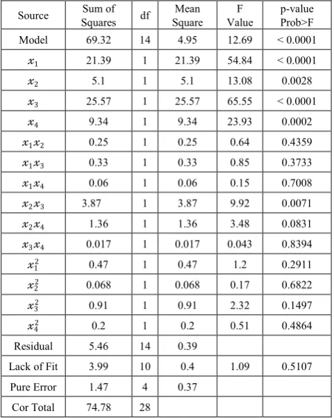
model fitting in the form of analysis of variance (ANOVA).The analysis of variance is essential to test significance and adequacy of the model. It subdivides the total variation of the results in two sources of variation, the model and the experimental error, shows whether the variation from the model is significant when compared to the variation due to residual error [28]. The Fisher’s F-test value, which is the ratio between the mean square of the model and the residual error, performs this comparison [29, 30]. If the model is a good predictor of the experimental results, F-value should be greater than the tabulated value of F-distribution for a certain number of degrees of freedom in the model at a level of significance. The F-value obtained, 12.69, is greater than the F value (2.47 at 95% significance) obtained from the standard distribution table, confirming the adequacy of the model fits. In addition, the p-value was found to be < 0.0001, which indicated that the model was highly statistically significant.
The ‘‘Lack of Fit Test’’ compares the residual error to the pure error from replicated design points. The "Lack of Fit F-value" of 1.09 implies the Lack of Fit is not significant relative to the pure error. There is a 51.07% chance of occurrence of noise, indicating significance of the model.
The significance of each term was determined by p-value (Prob>F), which is listed inTable 2.
As seen in this table that the terms 𝓍𝓍1 , 𝓍𝓍2 , 𝓍𝓍3 , 𝓍𝓍4 and 𝓍𝓍2𝓍𝓍3 ,were significant, with very small p-values (p < 0.05). The other term coefficients were not significant (p > 0.05).
The Pareto analysis [31] was carried out to check the percentage effect of each factor. In fact, this analysis calculates the percentage effect (𝒫𝒫𝒾𝒾) of each factor on the response, according to the following relation:
𝒫𝒫𝒾𝒾= �𝛽𝛽𝒾𝒾
2
∑ 𝛽𝛽𝒾𝒾2� × 100 (𝒾𝒾 ≠ 0) (10)
where 𝛽𝛽𝒾𝒾 is the regression coefficient of individual process variable.
Fig. 3 shows the Pareto graphic analysis. As can be seen in this figure, among the variables, the adsorbent dose (𝛽𝛽3 , 12.308% and𝛽𝛽32, 87.188%) produce the main effect on the adsorption capacity.
Figure 2. Comparison of the experimental results of adsorption capacity with those predicted via BBD model.
[image:4.595.313.548.76.231.2]Figure 3. Pareto graphic analysis.
Table 2. Analysis of variance (ANOVA) for Response Surface Quadratic Model
Source Squares Sum of df Square Mean Value F p-value Prob>F
Model 69.32 14 4.95 12.69 < 0.0001
𝓍𝓍1 21.39 1 21.39 54.84 < 0.0001
𝓍𝓍2 5.1 1 5.1 13.08 0.0028
𝓍𝓍3 25.57 1 25.57 65.55 < 0.0001
𝓍𝓍4 9.34 1 9.34 23.93 0.0002
𝓍𝓍1𝓍𝓍2 0.25 1 0.25 0.64 0.4359
𝓍𝓍1𝓍𝓍3 0.33 1 0.33 0.85 0.3733
𝓍𝓍1𝓍𝓍4 0.06 1 0.06 0.15 0.7008
𝓍𝓍2𝓍𝓍3 3.87 1 3.87 9.92 0.0071
𝓍𝓍2𝓍𝓍4 1.36 1 1.36 3.48 0.0831
𝓍𝓍3𝓍𝓍4 0.017 1 0.017 0.043 0.8394
𝓍𝓍12 0.47 1 0.47 1.2 0.2911
𝓍𝓍22 0.068 1 0.068 0.17 0.6822
𝓍𝓍32 0.91 1 0.91 2.32 0.1497
𝓍𝓍42 0.2 1 0.2 0.51 0.4864
Residual 5.46 14 0.39
Lack of Fit 3.99 10 0.4 1.09 0.5107 Pure Error 1.47 4 0.37
Cor Total 74.78 28
3.2. Artificial Neural Network
In order to determine the optimum number of neurons in the hidden layer, a series of topologies was examined. The mean square error (MSE) was used as the error function.It measures the performance of the network. Moreover, the
correlation coefficient (𝑟𝑟) was used as a measure of the predictive ability of the network. ANN optimization process required network training to minimize the error function (MSE) by searching for a set of connection weights that can enable the ANN to produce outputs that are identical or possibly equal to target values.
After repeated trials, it was found that a network with 11 hidden neurons produced the best performance. The optimal architecture of ANN model in this case is shown in Fig. 4. It 4 5 6 7 8 9 10 11
4 5 6 7 8 9 10 11
Actual qe (mg/g)
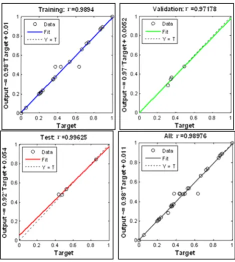
[image:4.595.312.553.264.565.2] [image:4.595.61.294.584.730.2]has three-layer ANN, with tangent sigmoid transfer function (tansig) at hidden layer with 11 neurons and linear transfer function (purelin) at output layer. The MSE value was found to be 0.0003 (Fig.5). A regression analysis between ANN outputs and the experimental data was carried out. This ANN model indicated a precise and effective prediction of the experimental data with a correlation coefficient (𝑟𝑟) of 0.989, 0.971, 0.996 and 0.989 for training, validation, testing and all data, respectively (Fig.6).
Figure.4. Optimal architecture of ANN model.
Figure.5. Evolution of network performance (MSE) during training phase using Levenberg–Marquardt backpropagation algorithm
The weights and biases associated with the final trained network are given in Table 3. The ANN model can be
presented mathematically as an input–output composite mapping:
Υ𝓃𝓃(X) = ϕ(2)�ℒ𝒲𝒲{2,1}ϕ(1)(ℐ𝒲𝒲{1,1}X + b{1}) + b{2}� (11) where 𝛶𝛶𝓃𝓃 denotes the vector of the normalized output (network predictions), 𝑋𝑋 is the vector of the input variables, 𝜙𝜙(1) is the vector of tansig transfer function corresponding to the hidden layer , 𝜙𝜙(2) is the vector of purelin transfer function corresponding to the output layer, ℐ𝒲𝒲{1,1} is the input weight matrix, ℒ𝒲𝒲{2,1} is the layer weight vector, 𝑏𝑏{1} is the bias vector, and 𝑏𝑏{2} is the bias scalar.
Figure.6. Network model with training, validation, test and all prediction set.
Table 3. Optimal values of the network weights and biases.
0 0.5 1 1.5 2 2.5 3 3.5 4 10-5
10-4 10-3 10-2
Best Validation Performance is 0.00030271 at epoch 1
M
ean
S
qu
ar
ed
E
rr
or
(
m
se)
4 Epochs
[image:5.595.315.551.225.488.2] [image:5.595.126.488.542.742.2]To evaluate the relative importance of the input variables on the Output variable (𝓆𝓆ℯ (mg/g)), neural net weight matrix and Garson equation were used in the evaluation processes. Garson proposed the equation based on the partitioning of connection weights as shown in Eq. (12) [27, 32-33]:
ℐ𝒾𝒾=
∑ �� �𝒲𝒲𝒾𝒾 𝓂𝓂𝒾𝒾 𝒽𝒽 �
∑𝒩𝒩𝒾𝒾𝓀𝓀=1�𝒲𝒲𝓀𝓀 𝓂𝓂𝒾𝒾 𝒽𝒽 ���𝒲𝒲𝓂𝓂 𝓃𝓃𝒽𝒽𝒪𝒪�� 𝒩𝒩𝒽𝒽
𝓂𝓂=1
∑ �∑ � �𝒲𝒲𝓀𝓀 𝓂𝓂𝒾𝒾 𝒽𝒽 �
∑𝒩𝒩𝒾𝒾𝓀𝓀=1�𝒲𝒲𝓀𝓀 𝓂𝓂𝒾𝒾𝒽𝒽 �� 𝒩𝒩𝒽𝒽
𝓂𝓂=1 �𝒲𝒲𝓂𝓂 𝓃𝓃𝒽𝒽𝒪𝒪��
𝒩𝒩𝒾𝒾 𝓀𝓀=1
(12)
where, ℐ𝒾𝒾 is the relative significance of the 𝒾𝒾th input variable on the output variable, 𝒩𝒩𝒾𝒾 and 𝒩𝒩𝒽𝒽 are the number of input and hidden neurons, respectively. 𝒲𝒲 is connection weight, the superscripts “𝒾𝒾” “𝒽𝒽” and “𝒪𝒪” represents the input, hidden, and output layers, respectively, while the subscripts “𝓀𝓀”, “𝓂𝓂” and “𝓃𝓃” refer to input, hidden, and output neurons, respectively.
[image:6.595.310.553.312.568.2]The relative significance (Table 4) of the four input variable computed by the Garson equation showed that all variables have strong effect on adsorption capacity (𝓆𝓆ℯ). Adsorbent dose and pH are the most significant variables with 38.24 and 26.11%, respectively, followed by the initial concentration of fluoride (19.49%), and finally the temperature (16.14%).
Table 4. Relative importance of input variables.
Input Variable Importance(%) Initial Concentration 19.49
pH 26.11
Adsorbent dose 38.24
Temperature 16.14
Total 100
3.3. Comparison of ANN and RSM Models
The comparison of RSM and ANN methodologies for predicted experimental results was done in terms of coefficient of determination (R2), root mean squared error
(RMSE) and average absolute deviation (AAD) which can be defined as follows:
𝑅𝑅𝑅𝑅𝑅𝑅𝑅𝑅 = �1𝓃𝓃∑ �𝑦𝑦𝓃𝓃𝒾𝒾=1 𝒾𝒾,𝑒𝑒𝑥𝑥𝑝𝑝 − 𝑦𝑦𝒾𝒾,𝑝𝑝𝑟𝑟𝑒𝑒𝑝𝑝�2� 1 2⁄
(14)
𝑅𝑅2= 1 −∑𝓃𝓃𝒾𝒾=1(𝑦𝑦𝒾𝒾,𝑝𝑝𝑟𝑟𝑒𝑒𝑝𝑝−𝑦𝑦𝒾𝒾,𝑒𝑒𝑥𝑥𝑝𝑝)2
∑𝓃𝓃𝒾𝒾=1(𝑦𝑦𝒾𝒾,𝑝𝑝𝑟𝑟𝑒𝑒𝑝𝑝−𝑦𝑦𝓂𝓂)2 (15)
𝐴𝐴𝐴𝐴𝐴𝐴 = ��∑ ��𝑦𝑦𝓃𝓃𝒾𝒾=1 𝒾𝒾,𝑝𝑝𝑟𝑟𝑒𝑒𝑝𝑝 − 𝑦𝑦𝒾𝒾,𝑒𝑒𝑥𝑥𝑝𝑝� 𝑦𝑦� 𝒾𝒾,𝑒𝑒𝑥𝑥𝑝𝑝�� 𝓃𝓃⁄ � × 100 (16) where 𝑦𝑦𝒾𝒾,𝑝𝑝𝑟𝑟𝑒𝑒𝑝𝑝 was the predicted value by ANN model, 𝑦𝑦𝑖𝑖,𝑒𝑒𝑥𝑥𝑝𝑝 was the experimental value, 𝓃𝓃 was the number of data, and 𝑦𝑦𝓂𝓂 was the average of the experimental value.
The comparative values RMSE, AAD, and R2 are given in
Table 5. The root mean squared error (RMSE) for the design matrix by RSM and ANN is 0.0942 and 0.0262, the coefficient of determination (R2) is 0.927 and 0.979, and the
absolute average deviation (AAD) is 5.110 and 1.320. The deviation of predicted response from experimental data (table1) for both methodologies is shown in Fig. 7. These results indicate that the ANN model showed a clear superiority over RSM for both data fitting and estimation capabilities. This higher predictive accuracy of ANN can be attributed to its universal ability to approximate nonlinearity of the system whereas RSM is only restricted to a second-order polynomial [34, 35]. In addition, it is to be noted that though RSM has the advantage of giving a regression equation for prediction and showing the effect of experimental factors and their interactions on response in comparison with ANN, ANN does not require a standard experimental design to build the model [23]. Another advantage of ANN model is flexible and permits to add new experimental data to build a trustable ANN model. In contrast, ANN methodology may require a greater number of experiments than RSM [23].
Table 5. Comparison of RSM and ANN.
Parameters Box-Behnken Design data
RSM ANN
RMSE 0.0942 0.0262
R2 0.927 0.979
AAD 5.110 1.320
Figure 7. The scatter plot of RSM and ANN model predicted values versus actual values for Box-Behnken design matrix.
4. Conclusion
In this study, the effects of pH, adsorbent mass, initial concentration, and temperature, on the adsorption capacity of fluoride onto apatitic tricalcium phosphate were investigated using RSM and ANN methods. The root mean square error(𝑅𝑅𝑅𝑅𝑅𝑅𝑅𝑅), coefficient of determination (𝑅𝑅2) and absolute average deviation (𝐴𝐴𝐴𝐴𝐴𝐴) were used together to compare the performance of the RSM and ANN models. The ANN model was found to have higher predictive capability than RSM model even with limited number of experiments.
4 5 6 7 8 9 10 11
4 5 6 7 8 9 10 11
Model Predicted (P)
Actual (A)
[image:6.595.59.298.392.496.2]Thus, it can be concluded that even though RSM is most widely used method for adsorption optimization, the ANN methodology may present a better alternative.
REFERENCES
[1] G.E.P Box, K.B.Wilson, On the Experimental Attainment of Optimum Conditions, Journal of the Royal Statistical Society B, 13, 1-45, 1951.
[2] R. H. Myers, D.C. Montgomery, Response Surface
Methodology: process and product optimization using designed experiment, A Wiley-Inter-science Publication, 2002.
[3] V .Gunaraj, N.Murugan , Application of response surface methodologies for predicting weld base quality in submerged arc welding of pipes, J. Mater. Process. Technol .,88,266–75, 1999
[4] G.E.P Box, D.W. Behnken, Some new three level designs for the study of quantitative variables, Technometrics, 2,455–475, 1960.
[5] R.H. Myers, D.C. Montgomery, Response surface
methodology: process and product optimization using designed experiments (1st ed.). New York: John Wiley & Sons, Inc,1995.
[6] X. Du, Q. Yuan , J. Zhao, Y. Li, Comparison of general rate model with a new model—artificial neural network model in describing chromatographic kinetics of solanesol adsorption in packed column by macroporous resins, Journal of Chromatography A, 1145, 165–174,2007.
[7] M.Sadrzadeh, T. Mohammadi, J.Ivakpour, N. Kasiri, Separation of lead ions from wastewater using electrodialysis: Comparing mathematical and neural network modeling. Chemical Engineering Journal, 144, 431–441,2008.
[8] S. Elemen , E. Perrin , A. Kumbasar , S. Yapar, Modeling the adsorption of textile dye on organoclay using an artificial neural network, Dyes and Pigments , 95,102-111,2012. [9] K. Moosavi , S. Setayeshi , M.Gh. Maragheh , S.J. Ahmadi ,
M.R. Kardan , L.M. Banaem. An optimization on strontium separation model for fission products (inactive trace elements) using artificial neural networks, Annals of Nuclear Energy , 36 , 1129–1132, 2009.
[10] A.R. Khataee , G. Dehghan , A. Ebadi , M. Zarei , M. Pourhassan. Biological treatment of a dye solution by Macroalgae Chara sp.: Effect of operational parameters, intermediates identification and artificial neural network modeling, Bioresource Technology, 101, 2252–2258, 2010. [11] M. Khajeh, M. G.Moghaddam, M. Shakeri, Application of
artificial neural network in predicting the extraction yield of essential oils of Diplotaenia cachrydifolia by supercritical fluid extraction,J. of Supercritical Fluids, 69 , 91– 96,2012. [12] S.M. Karazi, A.Issa,D.Brabazon,Comparison of ANN and
DoE for the prediction of laser-machined micro-channel
dimensions,Optics and Lasers in Engineering,47 ,956–964,2009.
[13] M. Khayet, C. Cojocaru, M. Essalhi, Artificial neural network modeling and response surface methodology of desalination by reverse osmosis, Journal of Membrane Science, 368, 202–214,2011.
[14] K. Sinha, S. Chowdhury, P. D. Saha, S. Datta, Modeling of microwave-assisted extraction of natural dye from seeds of Bixa orellana (Annatto) using response surface methodology (RSM) and artificial neural network (ANN), Industrial Crops and Products ,41,165– 171,2013.
[15] Ch.Y. Cheok, N. L. Chin, Y. A. Yusof, R. A. Talib, Ch. L. Law,Optimization of total phenolic content extracted from Garcinia mangostana Linn.hull using response surface methodology versus artificial neural network, Industrial Crops and Products, 40 , 247– 253,2012.
[16] M. Khajeh , M. Kaykhaii , A. Sharafi, Application of PSO-artificial neural network and response surface methodology for removal of methylene blue using silver nanoparticles from water samples, J. Ind. Eng. Chem.,http://dx.doi.org/10.1016/j.jiec.2013.01.033.
[17] H. Ebrahimzadeh , N.Tavassoli , O.Sadeghi ,
M.M.Amini.,Optimization of solid-phase extraction using artificial neural networks and response surface methodology in combination with experimental design for determination of gold by atomic absorption spectrometry in industrial wastewater samples. Talanta, 97, 211–217,2012.
[18] K. Sinhaa, P. D. Sahaa, S. Datta, Response surface optimization and artificial neural network modeling of microwave assisted natural dye extraction from pomegranate rind, Industrial Crops and Products, 37,408– 414, 2012. [19] A. K. Lakshminarayanan, V. Balasubramania, Comparison of
RSM with ANN in predicting tensile strength of friction stir welded AA7039 aluminium alloy joints, Trans. Nonferrous Met. Soc. China , 19, 9-18,2009.
[20] M. Khayet , C. Cojocaru, Artificial neural network model for desalination by sweeping gas membrane distillation, Desalination ,308 , 102–110,2013.
[21] [21] D. Bingol , M. Hercan , S. Elevli , E. Kılıc , Comparison of the results of response surface methodology and artificial neural network for the biosorption of lead using black cumin, Bioresource Technology ,112, 111–115,2012.
[22] Ranjan, D., D. Mishra, S.H.Hasan, Bioadsorption of arsenic: an artificial neural networks and response surface Methodological Approach. Ind. Eng. Chem. Res., 50, 9852–9863,2011.
[23] F.Geyikci, E. Kılıc, S. Coruh, S. Elevli, Modelling of lead adsorption from industrial sludge leachate on red mud by using RSM and ANN, Chemical Engineering Journal, 183 ,53– 59,2012.
[24] J. C. Heughebaert, PhD Thesis status, I.N.P, Toulouse, 1977. [25] M. Mourabet, A. El Rhilassi, H. El Boujaady, M. Bennani- Ziatni, R. El Hamri, A.Taitai, Removal of fluoride from aqueous solution by adsorption on Apatitic tricalcium phosphate using Box–Behnken design and desirability function, Appl. Surf. Sci. 258 ,4402-4410,2012.
[27] E.S. Elmolla, M. Chaudhuri, M. M. Eltoukhy, The use of artificial neural network (ANN) for modeling of COD removal from antibiotic aqueous solution by the Fenton process, Journal of Hazardous Materials, 179, 127–134,2010.
[28] J.Segurola, N. S. Allen, M. Edge, A. M. Mahon, Design of eutectic photoinitiator blends for UV/visible curable acrylated printing inks and coatings, Progress in Organic Coatings, 37 23-37,1999.
[29] M.B. Kasiri, N. Modirshahla , H.Mansouri , Decolorization of organic dye solution by ozonation; Optimization with response surface methodology, International Journal of Industrial Chemistry, 4:3, 2013 .
[30] A.R. Khataee, M. Fathinia, S. Aber, M. Zarei, Optimization of photocatalytic treatment of dye solution on supported TiO2 nanoparticles by central composite design: Intermediates identification, Journal of Hazardous Materials, 181, 886–897,2010.
[31] A.I. Khuri , J.A.Cornell , Response surfaces, 2nd edn. Dekker,
New York, 1996.
[32] G.D. Garson, Interpreting neural-network connection weights, A.I .Expert, 6, 47–5,1991.
[33] D. Salari, A. Niaei, A.R. Khataee, M. Zarei, Electrochemical treatment of dye solution containing C.I. Basic Yellow 2 by the peroxi-coagulation method and modeling of experimental results by artificial neural networks, J. Electroanal. Chem., 629, 117–125, 2009.
[34] P. Singh , S. S. Shera , J. Banik , R.M. Banik, Optimization of cultural conditions using response surface methodology versus artificial neural network and modeling of L-glutaminase production by Bacillus cereus MTCC 1305, Bioresource Technology, 137, 261–269,2013.