Abstract—This work presents a measurement campaign in a
complex urban propagation scenario in downtown Patras, Greece, where a community-based metropolitan area Wi-Fi/ WLAN operates at 2.4 GHz. Path loss and shadow fading characterization has been accomplished and the fine-tuning of respective models and distributions has taken place in order to compare empirical data with theoretical assumptions. These measurements have allowed for an extension of well-known path loss models from their established cellular-frequency operating range to the 2.4 GHz channel, and the relative mean error has been calculated for each model employed in our case study. Practical conclusions are derived, confirming, among others, the log-normal nature of shadow depth in an urban propagation environment for specific topology characteristics (road width, building separation, average building height).
Index Terms—path loss; shadowing; outdoor propagation;
metropolitan area network; urban topology; model fine-tuning
I. INTRODUCTION
IRELESS Channel Characterization consists of describing the quantitative and qualitative phenomena that alter the useful signal when transmitted over a wireless propagation link [1]. Signal attenuation, namely path loss, and fading due to shadow obstruction (large-scale) and multipath (small-scale), distort the signal amplitude and phase at the receiver [2]. The fundamental mechanisms of reflection, diffraction and scattering have been studied and investigated in a series of works in both outdoor and indoor propagation topologies [3]-[11].
Whereas in indoor propagation topologies we are mostly interested in describing in our mathematical formula all phenomena that influence signal propagation and attenuation to the best possible degree, in outdoor propagation case studies, the precise and reliable prediction of the average path loss and large-scale fading characterization remains an open issue [12]. Many textbooks and well-known research works deal with channel modeling and path loss calculation for the GSM-GSPRS-3G cellular frequency band (900 MHz, 1800 MHz, 2 - 2.1 GHz), investigated mostly during the 1990’s, when urban propagation modeling was very crucial in the context of micro-cellular design [13].
Manuscript received January 9, 2013; revised February 4, 2013. Theofilos Chrysikos is with the Department of Electrical and Computer Engineering, University of Patras, Patras, Greece (e-mail: [email protected]).
Stavros Kotsopoulos is with the Department of Electrical and Computer Engineering, University of Patras, Patras, Greece (phone: 00302610996466; e-mail: [email protected]).
Urban channel modeling and characterization, however, is not important only for cellular networks but also in higher frequencies of interest, for metropolitan and wide-area networks in the 2.4 GHz frequency (Wi-Fi/WLAN) as well as the WiMAX frequencies, i.e. 3.5 GHz. In addition, roadside and other vehicular-oriented applications at the 5 and 5.85 GHZ bands can also operate within the boundaries of an urban or suburban environment [14]. Thus, knowledge of the intrinsic channel characteristics, and the urban/suburban topology irregularities, and validation of their impact on the propagated electromagnetic waves, is highly critical for the design, implementation and operating evaluation of all these systems and applications [15].
In this work, a community-run metropolitan area Wi-Fi/WLAN operating at 2.4 GHz in downtown Patras, Greece is investigated [16]. In this urban propagation scenario, a measurement campaign has been conducted with the aid of a laptop equipped with an omni-directional antenna. Local mean power values have been recorded in various locations around the transmitting antenna, located on top of a building, and all topology characteristics (road width, building separation, average building height) for the area under investigation have been considered and incorporated in the validation of employed path loss models, including the urban formula of the Hata model and the Walfish-Ikegami model, two fundamental path loss models for urban areas for the cellular frequency band. For this case study, the path loss models have been employed outside their suggested frequency range. Mean error and deviation from the measured received power values are employed to evaluate the robustness of these models for the 2.4 GHz channel. In addition, the shadow depth according to Jakes [17] has been calculated and the Gaussian distribution has been employed for the logarithmic (dBm) values of the residue path loss in order to investigate the log-normal nature of large-scale fading due to shadow obstruction, as mentioned in other works of interest as well [18]-[22].
The paper is structured as follows: Section II presents the basic urban-area path loss models and their parameter limitations within the cellular frequency band. Section III describes the measurement campaign and the urban topology characteristics. Section IV presents the path loss models validation based on the measurements, whereas Section V describes the characterization of large-scale fading. Finally, Section VI sums up the conclusions and addresses future work issues in the area of wireless channel characterization for urban propagation topologies.
Site-specific Validation of Path Loss Models
and Large-scale Fading Characterization for a
Complex Urban Propagation Topology at 2.4
GHz
Theofilos Chrysikos and Stavros Kotsopoulos
II.OUTDOOR RFMODELS A.Path loss modeling
The reliable prediction of average path loss, and therefore of the local mean received power, throughout an urban topology, requires the employment of error-checked path loss models, that can range from the most simplistic and idealistic in terms of assumed propagation mechanisms, to the most elaborate, in terms of incorporating topology characteristics (building height, antenna height, road width) to the path loss formula.
In this work, three different path loss models will be validated: the Free Space model, which is theoretical and in fact a logarithmic expression of the Friis equation, assuming idealistic free space propagation, and two standard empirical models for urban areas, the Hata model and the Walfish-Ikegami model.
B.Free Space Model
As already mentioned, the Free Space model assumes that no obstacles or other terrain irregularities meddle with the signal path. The model does not consider any antenna height for either transmitter or receiver and idealistic propagation in three-dimensional plane is considered. The average path loss (in dB) is provided by the following formula [2]:
10 10
32.45 20 log
(
)
20 log
(
)
L
P
=
+
f MHz
+
d km
(1)The Free Space model can be applied to any given propagation topology as no distance or frequency limitations exist. The model assumes an inverse-square law for the attenuation of received power over distance.
C.Hata Urban Model
The Hata model [23] is a mathematical expression of the empirical model first developed by Okumura in the 1960’s [24]. Whereas the Okumura model was based on curves obtained from extensive measurements in urban areas in Japan, the Hata model, developed in 1980, allowed for an elaborate mathematical logarithmic formula [23]:
10 10
10 10
(
)
69.55 26.16 log
(
) 13.82 log
(
) (44.9 6.55 log
) log
(
)
L t
re t
P dB
f MHz
h
a h
h
d km
=
+
−
−
+
−
(2) Where
a h
(
re)
is a correction factor for the receiving antenna height, based on the topology and the channel characteristics. In our case,a h
(
re)
is provided by:
a h
(
re)
=
3.2 log (11.75
(
10h
re)
)
2−
4.97
(3)Where
h
t andh
reare the effective antenna heights for transmitter and receiver respectively, expressed in meters. The original Hata model is distance-bound (1-20 km) and frequency-bound (150-1500 MHz). Various extensions have been suggested, none however beyond the 2 GHz bound [13].D.Walfish-Ikegami Model
The Walfish-Ikegami path loss model is an elaborate path loss model for urban propagation topologies, originally developed for cellular bands (800 MHz – 2 GHz limitation) with a 5 km upper distance-bound [25]-[26].
In the case of an urban Line-of-Sight (LOS) scenario, the Free Space model is employed for d< 20 m, and beyond that the following formula applies:
P
L=
42.6 20 log
+
10f MHz
(
) 26 log
+
10d km
(
)
(4)In the Non-Line-of-Sight (NLOS) case:
P dB
L(
)
=
L dB
o(
)
+
L
rts(
dB
)
+
L
msd(
dB
)
(5)Where:
L
o represents free space loss and is provided by Eq. 1,L
rts is a correction factor representing diffraction and scattering from rooftop to street, andL
msd represents multi-screen diffraction due to urban rows of buildings. These terms vary with street width, building height and separation, angle of incidence.10 10
10
(
)
16.9 10 log
10 log
(
)
20 log (
)
rts
roof re ori
L
dB
w
f MHz
h
h
L
= −
−
+
+
−
+
(6)10
10 10
(
)
log
(
)
log
(
) 9 log
msd bsh a d
f
L
dB
L
K
K
d km
K
f MHz
b
=
+
+
+
−
(7)Where:
w
is the average street width,b
the average building separation,h
roof the building height andh
re the receiving antenna height, all expressed in meters.Since in our work a metropolitan center (downtown Patras, Greece) is considered and the transmitting antenna is on the rooftop of the building, namely
h
t >h
roof ,h
tbeing the transmitting antenna height expressed in meters, then54
aK
=
,K
d=
18
and the other parameters in Eq. 6 and 7 are provided by:
L
bsh(
dB
)
= −
18 log (1
10+ −
h
th
roof)
(8)
K
f= − +
4 1.5( / 925
f
MHz
−
1)
(9)In addition,
L
oriis provided by Table I as a function ofϕ
, defined as the road orientation with respect to direct radio path, expressed in degrees:TABLE I:LORI VALUES
10 0.354
ϕ
− +
if 0º ≤ϕ
≤ 35 º2.5 0.075(
+
ϕ
−
35)
if 35 º ≤ϕ
≤ 55 ºFig.1. Measurement site at downtown Patras, Greece.
III. MEASUREMENT SITE AND CAMPAIGN
Our set of measurements was conducted in downtown Patras, Greece, in one of the operating nodes of the Patras Wireless Network (PWN), a community-run metropolitan area network, involving many students of the Department of Electrical and Computer Engineering, and the Department of Computer Engineering and Informatics of the University of Patras, as well as self-taught local residents. PWN provides Wi-Fi and WLAN at 2.4 GHz (802.11b/g) for all users in the surrounding area of each node (within coverage range) and the backbone network of nodes runs at 5.2 GHz (802.11a).
This node and the neighbourhood, depicted in Fig.1, are located in the corner of Ellinos Stratiotou and Thessalonikis, in the center of Patras. A total of 19 measurements were conducted in the surrounding area. The received power value was detected and recorded in a laptop computer equipped with an omni-directional antenna of 2 dBi gain and the NetStumbler 0.40 software, which has already been validated as appropriate for measuring local mean values of received power in a given propagation topology at 2.4 GHz [27].
Measurements were conducted late at noon and repeated late at night, so that the body shadowing effect [28] would be minimized. In all cases, a time window of six minutes was allowed for each measurement, and an averaging of
10
λ
was performed around each location, so that small-scale phenomena would be discarded.IV. VALIDATION OF PATH LOSS MODELS
The transmitting node consisting of an omni-directional antenna with a total effective isotropic radiated power (EIRP) of 16 dBm. The building height was 14 m, whereas the effective transmitting antenna height was at 20 m. The receiving antenna height was 1 m (waist level), whereas the receiving antenna gain has been removed from all measured values in order to concentrate on the propagation channel (wireless interface between transmitter and receiver). All measurement locations provided a NLOS scenario. The average street width
w
was measured via GPS aid (latitude, longitude) and was found to be equal to 25 m approximately.Concerning the average building separation, it is commonly set equal to
2
w
, hence set to 50 m, which approximates the actual building separation in the buildings surrounding the transmitting node in Fig.1. A minimum mean square error (MMSE) estimation technique fit to the empirical data provided an optimal value of 64.56 meters for theb
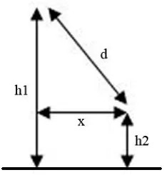
parameter, however it is usually considered to be upper-bound at 55 meters, with standard values around 50 m, as in our case.Fig.2. Precise calculation of T-R separation
Based on the horizontal distance
x
as defined in Fig.2, the angleϕ
was calculated for each measurement location, as shown in Table II. The area-mean angle, employed for the Walfish-Ikegami model, was found to beϕ
=
76.46
o.Based on these values of the aforementioned parameters, the mathematical expressions for the Free Space model, the Hata model and the Walfish-Ikegami model, allow for a fine-tuning of the Hata and Walfish-Ikegami model at 2.4 GHz, outside their frequency limitations.
P FS
r(
)
= −
84.05 20 log
−
10d km
(
)
(10)
P Hata
r(
)
= −
125.31 36.38 log
−
10d km
(
)
(11)
P WI
r(
)
= −
128.86 38 log
−
10d km
(
)
(12)TABLE II
ESTIMATION OF ANGLE
ϕ
x (m) φ( rad) φ ( º )
79.55 1.45 82.84
75.75 1.44 82.48
74.20 1.44 82.32
68.10 1.43 81.65
31.28 1.26 72.27
28.12 1.23 70.43
0.63 0.06 3.62
29.98 1.25 71.55
79.96 1.45 82.87
76.56 1.44 82.56
81.71 1.45 83.02
102.63 1.47 84.43
86.59 1.46 83.41
74.94 1.44 82.40
114.52 1.48 85.01
67.56 1.42 81.58
57.47 1.40 80.13
57.02 1.40 80.05
56.91 1.40 80.03
0 20 40 60 80 100 120
-95 -90 -85 -80 -75 -70 -65 -60 -55 -50
distance (m)
L
o
c
a
l
m
e
a
n
p
o
w
e
r
(d
B
m
)
[image:4.595.317.529.60.225.2]Measured values Free Space Hata Walfish-Ikegami
[image:4.595.111.226.62.185.2]Fig.3. Measured vs. Predicted values
Fig. 3 provides the measured values of local mean power versus the ones predicted by the employed path loss models. It is obvious that the Free Space model is inappropriate for this complex urban propagation topology as its predictions are unrealistically optimistic, based on the inverse-square law and discarding all obstacles and topology irregularities between transmitter and receiver.
On the other hand, the Hata model and the Walfish-Ikegami model provide much more reliable prediction for the local mean values of the received power, and perform quite similarly. Table III presents the relative error (%) for all employed models in each measurement location. Overall, the Free Space model has a mean error of 26.88%, the Hata Model has a mean error of 5.08% and the Walfish-Ikegami model a mean error of 5.2%.
TABLE III
RELATIVE ERRORS OF PATH LOSS MODELS
Loc.
T-R (m)
Pr (dBm)
Error % (FS)
Error % (Hata)
Error % (W-I)
A 82.03 -89 29.97 3.60 1.58
B 78.35 -87 28.82 2.21 0.19
C 76.85 -80 22.80 5.96 8.14
D 70.98 -77 20.68 8.46 10.65
E 37.13 -70 20.79 4.68 6.44
F 34.51 -77 28.82 6.34 4.80
G 20.01 -76 34.11 16.44 15.39
H 36.04 -75 26.42 2.93 1.31
I 82.42 -87 28.31 1.29 0.77
J 79.13 -91 31.85 6.34 4.40
K 84.12 -91 31.27 5.28 3.29
L 104.56 -93 30.71 3.62 1.51
M 88.87 -87 27.56 0.08 2.20
N 77.56 -78 20.71 8.87 11.11
O 116.25 -87 24.88 4.95 7.29
P 70.46 -77 20.77 8.31 10.50
Q 60.85 -80 25.33 1.35 3.33
R 60.43 -86 30.61 5.85 4.01
[image:4.595.74.257.457.779.2]V.LARGE-SCALE FADING
The large-scale variations of the average received signal over a given propagation environment, namely the local mean values of the received power, have been known to follow the log-normal distribution, the Probability Density Function (PDF) of which is given by [17]:
2 2
( ) 2
1
( )
2
x x
p x
e
σσ π
− −
=
(13)Where
x
is the received power (logarithmic value) in each measurement location (local mean strength),x
is the average received power (logarithmic value) for all measurement locations (mean value of the received power overall the topology in question), andσ
is the standard deviation of the shadowing losses (in dB).The large-scale variations of the received power have been attributed to losses by obstacles of proportions significantly larger than the signal wavelength, which remain constant over a time scale of seconds or minutes (large-scale fading). The shadowing deviation, or shadow depth, expresses the excess path loss, defined by Jakes as “the difference (in decibels) between the computed value of the received signal strength in free space and the actual measured value of the local mean received signal” [17].
To incorporate shadow fading losses and the large-scale fluctuations of the received signal power to the path loss formula, the Log-distance model is usually employed. The mathematical expression of the Log-distance path loss model is given by [12]:
0 10
0
(
)
log
total
d
L
PL d
N
X
d
σ
=
+
+
(14)Where
PL d
(
0)
is the path loss at the reference distance, usually taken as (theoretical) free-space loss at 100 m in classic cellular band scenarios,N
=
10
n
is the slope factor (wheren
is the path loss exponent) andX
σis a Gaussian random variable with zero mean and standard deviation ofσ
dB.N
andσ
are derived from experimental data.A fundamental problem with the Log-distance path loss model is that it requires a simultaneous attribution of values to various parameters. Even in the case of model fine-tuning, where a pool of measured local mean values of the received signal power are available, it is difficult to provide reliable values for all these parameters simultaneously. In addition, modifying the path loss exponent clearly distorts Jakes’ definition of the shadow depth and does not regard the shadow fading process as independent of distance-dependent free space propagation, a problem commonly met in both outdoor and indoor scenarios, as noted in [18]-[19]. Even worse, in the case of path loss prediction, where no pool of measured values exists, the log-distance model can be really difficult to implement without violating the definition of shadow depth by Jakes, thus altering the nature of the findings in regard to large-scale fading.
To overcome these obstacles, we fit the shadow depth
X
σto the measured data by assuming distance-dependent free space propagation with a path loss exponent ofn
=
2
. Thus, in each measurement location, we can calculate the shadow depth according to Jakes’ definition. Results are provided in Table IV. The shadow depthX
σhas an area-mean value of 22.35 dB and a deviation of 4.54 dB (or 4.66 dB if Bessel’s correction is employed).Fig. 4 depicts the cumulative distribution function (CDF) of these empirical values of the shadow depth, compared to the theoretical respective log-normal distribution (a Gaussian distribution is fit to the logarithmic values).
TABLE IV
SHADOW DEPTH VALUES
Loc. T-R (m)
Pr meas. (dBm)
Pr F-S (dBm)
Xs (dB)
A 82.03 -89 -62.33 26.67
B 78.35 -87 -61.93 25.07
C 76.85 -80 -61.76 18.24
D 70.98 -77 -61.07 15.93
E 37.13 -70 -55.44 14.56
F 34.51 -77 -54.81 22.19
G 20.01 -76 -50.07 25.93
H 36.04 -75 -55.19 19.81
I 82.42 -87 -62.37 24.63
J 79.13 -91 -62.02 28.98
K 84.12 -91 -62.55 28.45
L 104.56 -93 -64.44 28.56
M 88.87 -87 -63.03 23.97
N 77.56 -78 -61.84 16.16
O 116.25 -87 -65.36 21.64
P 70.46 -77 -61.01 15.99
Q 60.85 -80 -59.74 20.26
R 60.43 -86 -59.68 26.32
S 60.32 -81 -59.66 21.34
14 16 18 20 22 24 26 28 30
0 0.1 0.2 0.3 0.4 0.5 0.6 0.7 0.8 0.9 1
x
F
(x
)
Empirical vs. Theoretical CDF for Shadow Depth
Empirical Theoretical
VI. CONCLUSIONS
Several conclusions can be drawn from the findings above. First of all, it is demonstrated on the basis of the measured values of the local mean power of the received signal that both the Hata and the Walfish-Ikegami model can perform adequately even beyond their frequency limitations (1.5 GHz and 2 GHz respectively), for the 2.4 outdoor channel in an urban complex propagation topology, both providing a mean relative error marginally above 5%. On the other hand, an idealistic assumption as the one represented by the Free Space model is totally inappropriate for such a propagation environment.
In addition, it is quite remarkable that whereas both models perform in satisfactory fashion, the Hata model provides an equally reliable prediction as the more elaborate Walfish-Ikegami model. Calculating the average street width, the building separation and providing a precise estimation for the angle of incidence, parameters all required by the more complicated Walfish-Ikegami model, is certainly a much more time-consuming effort than the faster, on-the-fly urban formula of the Hata model. Even though the Hata model went further in terms of overriding the frequency limitation (from 1.5 GHz to 2.4 GHz), even though it does not incorporate as many parameters in its formula as the Walfish-Ikegami model, it predicts equally well (marginally better in this scenario). If this can be confirmed in other complex urban topologies for the 2.4 GHz channel, then the Hata model can be a fast and easy solution for path loss prediction in such environments.
Moreover, the shadow depth, as defined by Jakes based on the fluctuations of the large-scale fading due to shadow obstruction by buildings and other materials of significant dimensions compared to the signal wavelength, has been calculated empirically and it has been found to follow, indeed, the log-normal distribution (Gaussian fit to the logarithmic values), confirming similar findings in both outdoor and indoor scenarios.
Future work, focusing on more measurements in outdoor scenarios for the 2.4 GHz, will help further investigate the wireless channel characteristics and their impact on signal propagation and attenuation, as well as shadow fading characterization, for such topologies, which is of critical importance as metropolitan area networks are developing in the lower region of the SHF band.
REFERENCES
[1] A. Goldsmith, Wireless Communications. Cambridge: Cambridge University Press, 2005.
[2] J. D. Parsons, The Mobile Radio Propagation Channel. Hoboken, NJ: Wiley Interscience, 2000.
[3] C. Chrysanthou, H.L. Bertoni, “Variability of sector averaged signals for UHF propagation in cities”, in IEEE Transactions on Vehicular Technology, Volume 39, Issue 4, pp. 352–358, November 1990. [4] V. Erceg, L.J. Greenstein, S.Y. Tjandra, S.R. Parkoff, A. Gupta,
B. Kulic, A.A. Julius, R. Bianchi, “An Empirically Based Path Loss Model for Wireless Channels in Suburban Environments”, in IEEE Journal on Selected Areas in Communications, Volume 17, No. 7, July 1999.
[5] IEEE 802.16 Broadband Wireless Access Working Group, “Channel Models for Fixed Wireless Applications”, contribution to 802.16a, 2003.
[6] IEEE 802.11-03/940r4, “TGn Channel Models”, contribution to 802.11n, 2006.
[7] Y. Oda, R. Tsuchihashi, K. Tsunekawa, M. Hata, “Measured path loss and multipath propagation characteristics in UHF and microwave frequency bands for urban mobile communications” Vehicular Technology Conference, 2001. VTC 2001 Spring. IEEE VTS 53rd Volume 1, 6-9 May 2001 pp. 337-341 vol.1.
[8] J. S. Lee, L. E. Miller, CDMA Systems Engineering Handbook. Norwood, MA: Artech House, 1998.
[9] Recommendation ITU-R P.529-3, Prediction Methods for the Terrestrial Land Mobile Service in the VHF and UHF Bands, 1999. [10] K. W. Cheung, J. H. M. Sau, and R. D. Murch, “A new empirical
model for indoor propagation prediction”, IEEE Transactions on Vehicular Technology, vol. 47, no.3, pp. 996-1001, August 1998. [11] C. Oestges, P. Castiglione, N. Czink, “Empirical Modeling of
Nomadic Peer-to-Peer Networks in Office Environment”, IEEE Vehicular Technology Conference (VTC 2011-Spring), Budapest, Hungary, May 15-18, 2011.
[12] J. Seybold, Introduction to RF Propagation. Hoboken, NJ: Wiley Interscience, 2005.
[13] T. Rappaport, Wireless Communications: Principles & Practice. Upper Saddle River, NJ: Prentice Hall, 1999.
[14] D. W. Matolak, Q. Wu, I. Sen, “5 GHz Band Vehicle-to-Vehicle Channels: Models for Multiple Values of Channel Bandwidth,” IEEE Trans. Vehicular Tech., vol. 59, no. 5, pp. 2620-2625, June 2010. [15] D. W. Matolak, “Channel Modeling for Vehicle-to-Vehicle
Communications,” IEEE Communications Magazine (special section on Automotive Networking), vol. 46, no. 5, pp. 76-83, May 2008. [16] http://www.patraswireless.net/index.html
[17] W. C. Jakes (Ed.), Microwave mobile communications. New York, NY: Wiley Interscience, 1974.
[18] J. Salo, L. Vuokko, H. M. El-Sallabi, and P. Vainikainen, “An additive model as a physical basis for shadow fading”, IEEE Transactions on Vehicular Technology, vol.56, no.1, pp. 13-26, January 2007.
[19] T. Chrysikos, G. Georgopoulos, and S. Kotsopoulos, “Empirical calculation of shadowing deviation for complex indoor propagation topologies at 2.4 GHz”, International Conference on Ultra Modern Telecommunications (ICUMT 2009), St. Petersburg, Russia, October 12-14, 2009.
[20] T. Chrysikos, G. Georgopoulos, and S. Kotsopoulos, “Impact of shadowing on wireless channel characterization for a public indoor commercial topology at 2.4 GHz”, 2nd International Congress on Ultra
Modern Telecommunications (ICUMT 2010), Moscow, Russia, October 18-20, 2010.
[21] T. Chrysikos, G. Georgopoulos, and S. Kotsopoulos, “Wireless channel characterization for a home indoor propagation topology at 2.4 GHz”, Wireless Telecommunications Symposium 2011 (WTS 2011), New York City, USA, April 13-15, 2011.
[22] T. Chrysikos and S. Kotsopoulos, “Characterization of large-scale fading for the 2.4 GHz channel in obstacle-dense indoor propagation topologies”, IEEE Vehicular Technology Conference (VTC-Fall 2012), September 3-6, 2012, Quebec City, Canada.
[23] M. Hata, “Empirical Formula for Propagation Loss in Land Mobile Radio Services”, in IEEE Transactions on Vehicular Technology, Volume 29, No 3, pp. 317–325, August 1980.
[24] Y. Okumura, E. Ohmori, T. Kawano, K. Fukuda, “Field strength and its variability in VHF and UHF Land-Mobile radio service”, in Review of the Electrical Communication Laboratory, Volume 16, No. 9-10, pp. 825–873, September-October 1968.
[25] F. Ikegami, S. Yoshida, T. Takeuchi, M. Umehira, “Propagation Factors Controlling Mean Field Strength on Urban Streets”,in IEEE Transactions on Antennas & Propagation, Volume AP-32, pp. 822–829, 1984.
[26] J. Walfish, H.L. Bertoni, “A theoretical model of UHF propagation in urban environment, in IEEE Transactions on Antennas & Propagation, Volume AP- 36, pp. 1788–1796, December 1988. [27] T. Chrysikos, G. Georgopoulos, and S. Kotsopoulos, “Site-specific
validation of ITU indoor path loss model at 2.4 GHz”, 4th IEEE Workshop on Advanced Experimental Activities on Wireless Networks and Systems, Kos Island, Greece, June 19, 2009.