New Approach for Fuzzy Control and Analysis of Queueing System with Flexible Service Time

New Approach for Fuzzy Control and Analysis of

Queueing System with Flexible Service Time

Zafar Zafari, Javad Tavakoli

Abstract1– Fuzzy control of queues is a new method for controlling cost of the system, number of customers waiting in the queue and many other aspects of queues. This paper proposes fuzzy control approach for reducing cost of the system.

M

/

F

/

1

(Poisson arrival and fuzzy service rate) with flexible service time is examined in this paper. All the fuzzy mathematics rules in this paper are based on Zadeh’s extension principle, Mamdani implication, possibility and probability concept. At the end of this paper a simple numerical example is presented.

I. INTRODUCTION

Queueing theory is a classical mathematical method for studying the queues such as average waiting time and average number of customers in the system [2], [3]. Fuzzy queueing and fuzzy control of queues would be a new approach for surveying the queueing systems. If we let service time be expressed by possibility rather than probability, then fuzzy queueing method would be a more realistic approach than classical queueing theory methods.

1

/

/

F

M

(Poisson arrival and fuzzy service rate) with flexible service time is examined in this paper, and the objective is to employ a fuzzy policy to reduce the costs of the system and control the average number of customers in the queue. All the fuzzy mathematics rules in this paper are based on Zadeh’s extension principle [1], Mamdani implication, possibility and probability concept. The results of this paper can be extended to other queueing systems.

II.

M

/

F

/

1

QUEUES IN FUZZY ENVIROMENT Consider we have a queueing system with Poisson arrival, one server and fuzzy service time. The arrival rate is

λ

and the discipline is first in first served. Suppose that the service time is a fuzzy set denoted by

S

~

. Therefore

S

~

=

{

t

∈

ℜ

+

,

µ

_s

(

t

)

>

0

}

. Imagine after each service completion we have a new state. The number of customers that a person whose service is just completed

Manuscript received January 07, 2011.

Zafar Zafari is graduate student in department of Mathematics at University of British Columbia, 3333 University Way, Kelowna, BC, Canada, V1V 1V7 (email: [email protected]).

Javad Tavakoli is associate professor in department of Mathematics at University of British Columbia, 3333 University Way, Kelowna, BC, Canada, V1V 1V7 (email: [email protected]).

sees in the system is considered as a state of the system. Therefore the Probability that we move from state

i

to

j

is identical to the probability that

j

−

i

+

1

customers enter the system during the service time

t

. The probability of

i

arrivals during service time

t

is denoted by

P

~

_i. So this is a Markov chain and since all the probabilities are fuzzified, it’s considered as fuzzy Markov chain. We can show this fuzzy Markov chain as follows [5]:













































=

.

.

.

.

.

.

.

.

.

.

.

.

.

.

.

.

.

.

.

.

.

.

.

.

.

~

~

0

0

.

.

.

~

~

~

0

.

.

.

~

~

~

~

.

.

.

~

~

~

~

~

1 0 2 1 0 3 2 1 0 3 2 1 0

P

P

P

P

P

P

P

P

P

P

P

P

P

P

_ij

We need to solve the stationary equations. The stationary equations are as follows:

0

~

P

π

₀+

P

~

₀

π

₁=

π

₀,

P

~

₁

π

₀+

P

~

₁

π

₁+

P

~

₀

π

₃=

π

₁and so on. The results are as follows:

,

1

0

λ

t

π

=

−

[

exp(

)

1

]

)

1

(

1

=

−

λ

t

λ

t

−

π

,

2

,

)!

1

(

)

(

)!

(

)

(

)

exp(

)

1

(

)

1

(

1 1

≥













−

−

+

−

×

−

−

=

− − − = −

∑

n

k

n

t

k

k

n

t

k

t

k

t

k n k n n k k n n

λ

λ

λ

λ

π

i

and therefore

)

1

(

2

)

2

(

t

t

t

L

W

λ

λ

λ

−

−

=

=

.

We understand from above formulas that

L

and

W

are also fuzzy sets. So,













−

−

=

,

(

)

)

1

(

2

)

2

(

t

t

t

t

L

_λ

µ

s

λ

λ

and













−

−

=

,

(

)

)

1

(

2

)

2

(

t

t

t

t

W

_λ

µ

s

λ

III. FUZZY CONTROL

In this part we want to employ a policy to control the service time of queueing system in fuzzy environment. As Heyman has proved the optimal policy for costs, we just keep the server on as long as there is at least one customer in the system [4]. When system gets empty we turn the server off and the only thing we need to specify is when turn the server on. Suppose that in our system we have switching cost denoted by

SC

(whenever we turn the server on), Holding cost rate per customer (

HC

) and server running cost rate (

RC

). Also suppose that we have a flexible server which can switch from one service time to another one. The important fact in the real world is that running cost rate depends on the service rate (higher service rate=higher service running cost). So we should try to employ a policy to control the service time after turning on the server. Our fuzzy controller has two

outputs. One is

d

₁which indicates whether or not the server is on and the other is

d

₂which determines the service time. Now we need to know our inputs to be able to define our control logic.

If there is no switching cost , obviously it will be optimal to turn the server on as soon as one customer enters to the system. But since we have a big switching cost in most of the cases, we turn the server on when the accumulated holding cost (

AHC

)gets big enough to comptete with switching cost (

SC

):

∑

=

i

i

HCS

AHC

,

where

S

_iis the number of customers in the system in the

ith

unit of time.

Since we have the average arrival rate

λ

, therefore after first unit time we have average

λ

customers in the system. The average accumulated holding cost after first unit of time will be

AHC

=

HC

λ

/

2

. After

n

units of time the average accumulated holding cost will be

2

/

2

/

)

1

2

(

...

2

/

5

2

/

3

2

/

2

_HC

n

HC

n

HC

HC

HC

AHC

λ

λ

λ

λ

λ

=

−

+

+

+

+

=

.

Since when

AHC

gets equal to switching cost

SC

, we turn the server on (

d

₁is on), therefore

.

2

2

/

2

HC

SC

n

SC

HC

n

λ

[image:2.612.118.496.492.738.2]

λ

=

→

=

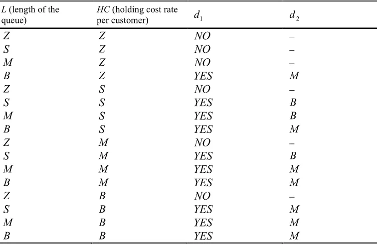
TABLE I. Rule base

L (length of the queue)

HC (holding cost rate

per customer)

d

1

d

2

Z

Z

NO

−

S

Z

NO

−

M

Z

NO

−

B

Z

YES

M

Z

S

NO

−

S

S

YES

B

M

S

YES

B

B

S

YES

M

Z

M

NO

−

S

M

YES

B

M

M

YES

M

B

M

YES

M

Z

B

NO

−

S

B

YES

M

M

B

YES

M

So when accumulated holding cost gets equal to length of the queue is approximately

HC

SC

n

L

λ

λ

λ

=

2

=

.

Therefore when the queue length is

λ

2

SC

turn the server on (

d

₁

=

on

). Also we know that higher the

h

, the easier it is to make a decision to turn the server on.

Now we should define the membership function of and

d

₂(service time). We computed that when length of the queue gets

λ

2

SC

λ

HC

we turn the dormant server on. So

λ

2

SC

λ

HC

is considered

our normalized interval is [

0

,

6

], we should scale

HC

SC

λ

λ

2

to

6

, so the scaling factor will

HC

SC

λ

λ

2

6

.

FIGURE I. Membership function: normalized input variable

hen accumulated holding cost gets equal to

SC

, the

HC

SC

λ

, we ). Also we know that the , the easier it is to make a decision to turn the

we should define the membership function of

h

,

L

time). We computed that when length of rn the dormant

BIG

. Since ], we should scale , so the scaling factor will be

The scaling factor for

HC

is

6

SC

functions for

L

and

HC

will be like figure I and II, respectively.

We computed

)

1

(

2

)

2

(

~

t

t

t

P

i

L

i

i

_λ

λ

λ

−

−

=

=

∑

.

The service time (

t

) by which

HC

SC

λ

λ

2

_{), is also considered}

should solve the following equation, which is

)

1

(

2

)

2

(

t

t

t

λ

λ

λ

−

−

HC

SC

λ

λ

2

=

.

We denote bigger

t

we get from above equation by and consider it as

BIG

. Therefore the scaling factor for

2

d

is

6

A

(figure III).

. Membership function: normalized input variable

L

SC

. The membership be like figure I and II,

L

_is

BIG

(

L

=

is also considered as

BIG

. So we should solve the following equation, which is:

we get from above equation by

A

FIGURE II. Membership function: normalized input

FIGURE III. The

IV. NUMERICAL EXAMPLE Suppose that we have a queueing system

M

arrival rate

λ

=

1

, holding cost rate

h

=

88

switching cost

SC

=

100

. Suppose that the length of the queue is

1

(

L

=

1

). The scaling factor for

SC

/

6

. So

88

.

88888

_{is scaled down to}

333333

.

5

100

6

88888

.

88

×

_≈

.

Also the scaling factor for

L

is

. Membership function: normalized input

HC

The Membership function: normalized output

d

₂

1

/

/

M

M

with

88888

.

88

and

. Suppose that the length of the . The scaling factor for

HC

is

4

2

6

=

HC

SC

λ

λ

.

So

L

=

1

is scaled to

4

.

According to figure II,

HC

=

5

.

with grade

0

.

33333

and is

BIG

Also from figure I, we understand that

MEDIUM

_{with grade}

1

.

d

₁ will be outputs are

YES

. From table 1 Mamdani implication we have the follow

3333

.

is

MEDIUM

If

HC

_is

MEDIUM

_{with grade}

0

.

33333

_and

L

is

MEDIUM

with grade

1

, then

d

₁ is

YES

_{with grade}

33333

.

0

.

If

HC

_is

BIG

with grade

0

.

66666

_and

L

_is

MEDIUM

_{with grade}

1

, then

d

₁ is

YES

_{with grade}

6666

.

0

. Because all the decisions on

d

₁ is

YES

, then the final decision on

d

₁ is also

YES

.

[image:5.612.69.267.462.721.2]

According to Mamdani implication and fuzzy rule base in table 1, the decision on

d

₂(service time) is as follows: If

HC

_is

MEDIUM

_{with grade}

0

.

33333

_and

L

is

MEDIUM

_{with grade}

1

, then

d

₂ is

MEDIUM

_with grade

0

.

33333

.

If

HC

_is

BIG

_{with grade}

0

.

6666

_and

L

_is

MEDIUM

_{with grade}

1

, then

d

2

is

MEDIUM

_with

grade

0

.

6666

.

According to figure III and above decisions, the peak values and heights of the fuzzy set are as follows:

e

₁

=

3

,

3

2

=

e

,

f

₁

=

0

.

33333

,

f

₂

=

0

.

6666

. Now by the height method of defuzzification, our final decision on

2

d

is

3

99

.

2

2

1

2

=

=

≈

∑

=

i

i i i

f

e

f

d

.

This is a normalized service time (

t

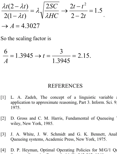
). For computing the original service time:

3027

.

4

5

.

1

2

2

2

2

)

1

(

2

)

2

(

2

=

→

=

−

−

→

=

−

−

A

t

t

t

HC

SC

t

t

t

λ

λ

λ

λ

λ

.

So the scaling factor is

.

15

.

2

3945

.

1

3

3945

.

1

6

=

=

→

=

t

A

REFERENCES

[1] L. A. Zadeh, The concept of a linguistic variable and its application to approximate reasoning, Part 3. Inform. Sci. 9, 43-64, 1975.

[2] D. Gross and C. M. Harris, Fundamental of Queueing Theory, wiley, New York, 1985.

[3] J. A. White, J. W. Schmidt and G. K. Bennett, Analysis of Queueing systems, Academic Press, New York, 1975.

[4] D. P. Heyman, Optimal Operating Policies for M/G/1 Queueing Systems, Operation Research, 16 (2), 362-382, 1968.