doi:10.4236/wet.2011.23025 Published Online July 2011 (http://www.SciRP.org/journal/wet)
Effect of Changes in Sea-Surface State on
Statistical Characteristics of Sea Clutter
with
X-band Radar
Seishiro Ishii1, Syuji Sayama1, Koichi Mizutani2
1Department of Communications Engineering, National Defense Academy, Yokosuka, Japan; 2Department of Intelligent Interaction Technology, University of Tsukuba, Tsukuba, Japan.
Email: [email protected]
Received March 9th, 2011; revised April 15th, 2011; accepted May 3rd, 2011.
ABSTRACT
We have made observations of X-band radar sea clutter from the sea surface and sea-surface state in the Uraga Suido Traffic Route, which is used by ships entering and leaving Tokyo Bay, and the nearby Daini Kaiho Sea Fortress. We estimated the distributions of reflected amplitudes due to sea clutter using models that assume Weibull, Log-Weibull, Log-normal, and K-distributions. We then compared the results of estimating these distributions with sea-surface state data to investigate the effects of changes in the sea-surface state on the statistical characteristics of sea clutter. As a result, we showed that observed sub-ranges not containing a target conformed better to the Weibull distribution re-gardless of Significant Wave Height (SWH). Further, sub-ranges conforming to the Log-Weibull or Log-normal distri-bution in areas contained a target when the SWH was large, and as SWH decreases, sub-ranges conforming to a Log-normal. We also showed that for observed sub-ranges not containing a target, the shape parameter, c, of both Weibull and Log-Weibull distribution correlated with SWH. The correlation between wave period and shape parame-ters of Weibull and Log-Weibull distribution showed a weak correlation.
Keywords: X-Band Radar, Sea Clutter, Significant Wave Height, Weibull Distribution, Log-Normal Distribution
1. Introduction
As electronics technology has advanced, equipment sup- porting marine navigation has become computerized, and highly automated vessels have begun to appear. Safe, reliable, and rapid goods delivery services are essential for a plentiful and comfortable society. To provide these services efficiently, cargo vessels are expected to in-crease in size, speed and energy efficiency, and ensuring the safe navigation of these vessels is an important issue. Sea charts are also essential for safe navigation, and Elec-tronic Chart Display and Information Systems (ECDIS) [1] have been realized, able to display radar data overlaid on the charts. This has contributed to radar becoming essen-tial for safe navigation of sea vessels.
The signal received by radar contains reflections from various objects besides the intended targets, such as land, clouds, rain, and the sea surface. All such undesired re-flections from non-targets are referred to as clutter. The presence of this sort of clutter can result in false detec-tion of targets or undetected targets, and is a major ob-
stacle to target detection [2]. In order to suppress this clut-ter and detect targets accurately it is necessary to process the signals to obtain a Constant False Alarm Rate (CFAR), and to accomplish this, it is very important to study the statistical characteristics of clutter, such as the distribu-tion of reflected amplitudes, in detail [2-8].
The reflected-clutter amplitude distribution differs de-pending on what type of objects create the reflection, and reflections from land are called ground clutter, from rain and clouds are called weather clutter, and from the sea surface are called sea clutter [2].
taken observations of sea clutter and sea-surface state and compared them statistically to study the effects of sea-surface state on the statistical characteristics of sea clutter.
The paper is organized as follows: In Section 2, we in-dicate the observations which is included the sea state and the radar observations indicating the observation parameters. A solution to the sea clutter distribution as-sumptions and the distribution estimation are given in Section 3, and the effect on the reflected amplitude dis-tribution by changes in the sea surface is discussed in Section 4.
2. Observations
We conducted observations of the sea-surface state at the same time as taking radar measurements. The radar observations were made in areas including the busy Tokyo Bay Uraga Suido Traffic Route and the Daini Kaiho Sea Fortress. The Daini Kaiho Sea Fortress is a fortification initially built on the water at the entrance to Tokyo Bay as part of the captial’s defenses, but it is now a facility for ensuring the safety of vessels passing through the Uraga Suido Traffic Route, with equipment such as lighthouses and beacons, and also instruments for measuring the sea state. The observations were taken between April 2, and December 3, 2010, includ-ing a total of 106 data points. Radar data obtained dur-ing rain was excluded from the study because it in-cludes weather clutter from raindrops in addition to sea clutter. We also excluded data containing targets (ships, etc.) in the specified range where used for analyzing the statistical characteristics of sea clutter. We then assigned an observation number to each of the remain-ing 65 data points used for the study.
2.1. Sea State Observations
Significant wave height (SWH) and wave period data was extracted from ocean wave and the significant wave state data at the Tokyo Bay Daini Kaiho Sea Fortress from the National Ocean Wave information network for Ports and HArbourS (NOWPHAS) [10].
2.2. Radar Observations
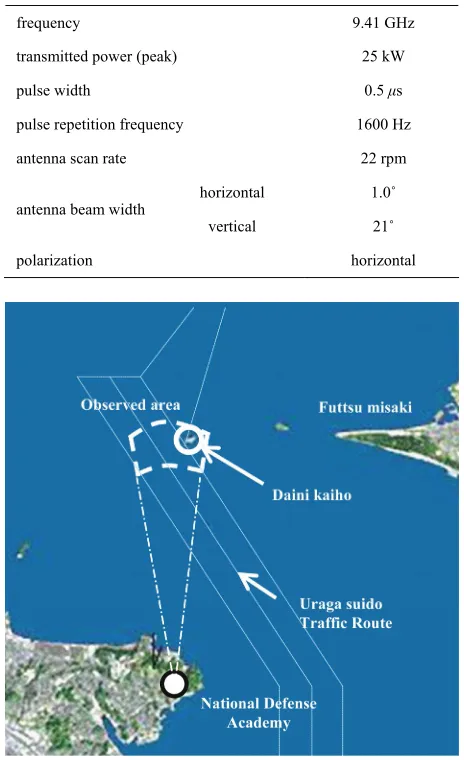
The region was observed using X-band radar equipment installed on the roof top at the National Defense Acad-emy in Yokosuka City. The main parameters of the X- band radar are given in Table 1. Figure 1 has an aerial
[image:2.595.307.539.99.479.2]photograph of the area around Tokyo Bay Uraga Suido Traffic Route showing the approximate region of the radar images taken as observation data with a dashed line. The extracted data covered an azimuth range sweep of 355.5˚ to 18.0˚ and distance range from 4.0 to 6.0 km, in the Uraga Suido Traffic Route surrounding the Daini
Table 1. X-band radar parameters.
frequency 9.41 GHz
transmitted power (peak) 25 kW
pulse width 0.5 μs
pulse repetition frequency 1600 Hz
antenna scan rate 22 rpm
horizontal 1.0˚ antenna beam width
vertical 21˚
polarization horizontal
Figure 1. Observed area.
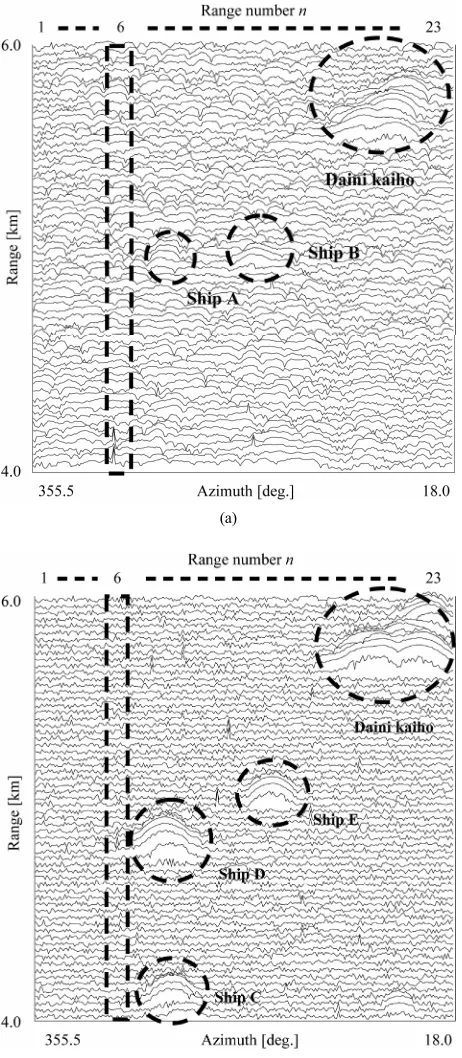
Kaiho Sea Fortress. 273 sweeps of the azimuth range were made. The antenna is installed 90 m above sea level, so the grazing angle was 1.4˚. 256 points on each of the range and azimuth axes were taken, totaling 65,536 data points, and the reflection amplitude at each point was quantized to 256 levels, from 0 to 255. As examples of this observed data, data from when the SWH was high (1.27 m) is shown in Figure 2(a) (observation number 64,
Dec. 3), and when the SWH was low (0.21 m) is shown in Figure 2(b) (observation number 21, Apr. 26). When
(a)
[image:3.595.58.289.84.613.2](b)
Figure 2. Observed data. (a) Significant wave height of 1.27 m; (b) Significant wave height of 0.21 m.
and leaving vessels passing through it and no reflective objects other than waves. The bump shapes shown sur-rounded by circles are radar targets: vessels passing through the Uraga Suido Traffic Route (Ships A to E) and the Daini Kaiho Sea Fortress.
3. Clutter Distribution Assumptions
We then tested conformity to the assumed distributions using the observation data for when the SWH was large and small, as shown in Figure 2(a) and (b) respectively.
Reference [11] gives a method for estimating parameters for a random variable according to various distributions as well as the expected values. In this study, we mated the parameters using a maximum likelihood esti-mator.
3.1. Assumed Distribution Models
Sea clutter reflection amplitude distributions have been reported to follow K, Weibull, Log-Weibull, and Log- normal distributions [12], and these have all been studied for use in implementing CFAR [2]. However, there is a known problem [12] with the K-distribution, which is expressed in terms of shape (v) and scale (h) parameters. When sections of the reflected clutter amplitude prob-ability are large, and get larger than a Raleigh distribu-tion (a Weibull distribudistribu-tion with shape parameter of 2), the value of v goes to infinity and it is not possible to calculate the probability density. Thus, when assuming a K-distribution model it was not possible to estimate the distribution for sub-ranges not containing a target, re-gardless of the SWH, as is shown by the error marks in
Tables 2 and 3.
A Weibull distribution can be expressed by the fol-lowing probability density function.
1
exp
0, 0, 0
c c
W
c x x
p x
b b b
x b c
(1)
The Log-Weibull distribution is expressed by the fol-lowing probability density function.
1
ln ln
exp
1, 0, 0
c c
LW
c x x
p x
bx b b
x b c
(2)
where, x is the reflected amplitude, b is the scale pa-rameter and c is the shape papa-rameter.
The Log-normal distribution is given by the following probability density function.
2 ln
1 exp 1 2 2π
0, 0
L N
x
p x
x x
(3)
[image:3.595.334.540.628.677.2]varied.
1
1 4
2 ( )
0, 0, 0
k
h
p x x k hx
x h
(4) The Log-Weibull distribution is positioned between the Weibull and Log-normal distributions [2].
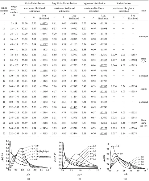
As the highest parts of the reflected clutter amplitude get higher, the Weibull and Log-Weibull distributions tend toward those with higher shape parameter (c) values, and the Log-normal distribution toward shapes with a smaller standard distribution, σ.
where, kν-1 is a modified Bessel function, and its parame-ters are a scale parameter, h, and a shape parameter, ν.
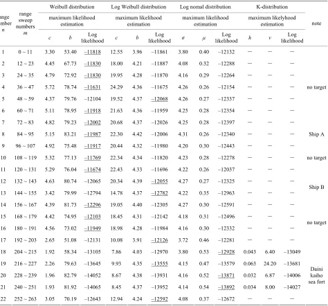
For reference, Figure 3(a) shows the changes in the
shape of the Weibull distribution when b is fixed and the shape parameter, c, is varied, Figure 3(b) shows how the
Log-normal distribution changes when the mean, μ, is fixed and the standard deviation, σ, is varied, and Figure 3(c) shows how the K-distribution changes when the
scale parameter,h, is fixed and the shape parameter, v, is
3.2. Beam Width and Sub-Ranges
[image:4.595.65.539.279.721.2]It is generally thought that reflected radar signals are strongly correlated within the antenna beam width, and have similar characteristics [2]. Thus, we divided the
Table 2. Result of distribution estimation for different range numbers at significant wave height of 1.27 m (observation num-ber 64).
Weibull distribution Log Weibull distribution Log nomal distribution K-distribution
maximum likelihood estimation
maximum likelihood estimation
maximum likelihood estimation
maximum likelyhood estimation range
number
n
range sweep numbers
m
c b likelihood Log c b likelihoodLog σ μ likelihoodLog h ν likelihoodLog
note
1 0 ~ 11 3.30 53.40 –11818 12.55 3.96 –11861 3.80 0.40 –12132 - - -
2 12 ~ 23 4.45 67.73 –11830 18.00 4.21 –11887 4.08 0.32 –12288 - - -
3 24 ~ 35 4.79 72.92 –11830 19.95 4.28 –11870 4.16 0.29 –12264 - - -
4 36 ~ 47 5.72 78.74 –11631 24.29 4.36 –11675 4.26 0.26 –12154 - - -
5 48 ~ 59 4.37 79.76 –12104 19.52 4.37 –12068 4.26 0.27 –12337 - - -
6 60 ~ 71 5.11 78.95 –11918 21.63 4.36 –11959 4.25 0.28 –12354 - - -
7 72 ~ 83 4.82 79.23 –12002 20.68 4.37 –12026 4.25 0.28 –12397 - - -
no target
8 84 ~ 95 5.15 83.21 –11987 22.30 4.42 –12006 4.31 0.26 –12340 - - - Ship A
9 96 ~ 107 4.92 75.48 –11917 20.44 4.32 –11980 4.20 0.30 –12443 - - -
10 108 ~ 119 5.32 77.13 –11769 22.34 4.34 –11820 4.23 0.28 –12278 - - -
11 120 ~ 131 5.29 76.04 –11674 22.43 4.33 –11696 4.22 0.26 –12037 - - -
no target
12 132 ~ 143 4.63 80.74 –12065 20.34 4.39 –12055 4.27 0.27 –12325 - - -
13 144 ~ 155 3.42 79.99 –12794 14.78 4.37 –12782 4.22 0.35 –12963 - - - Ship B
14 156 ~ 167 4.39 81.73 –12296 19.05 4.40 –12305 4.27 0.30 –12591 - - -
15 168 ~ 179 4.42 74.95 –12103 18.45 4.31 –12142 4.18 0.31 –12496 - - -
16 180 ~ 191 4.56 73.02 –11949 18.98 4.28 –11984 4.16 0.30 –12332 - - -
17 192 ~ 203 2.65 51.08 –12131 10.08 3.91 –12126 3.72 0.46 –12281 - - -
no target
18 204 ~ 215 1.92 58.34 –13105 7.86 4.03 –12970 3.80 0.53 –12928 0.043 6.40 –13049
19 216 ~ 227 2.26 79.63 –13645 9.93 4.35 –13555 4.15 0.47 –13579 0.063 24.20 –13681
20 228 ~ 239 1.96 82.79 –14052 8.67 4.38 –13931 4.16 0.52 –13871 0.032 6.87 –14006
21 240 ~ 251 1.93 81.92 –14065 8.45 4.37 –13952 4.14 0.54 –13892 0.034 8.00 –14027
22 252 ~ 263 3.05 70.19 –12643 12.94 4.24 –12592 4.08 0.37 –12672 - - -
Table 3. Result of distribution estimation for different range numbers at significant wave height of 0.21 m (observation num-ber 21).
Weibull distribution Log Weibull distribution Log nomal distribution K-distribution
maximum likelihood estimation maximum likelihood estimation maximum likelihood estimation maximum likelyhood estimation range number n range sweep numbers m
c b likelihood Log c b likelihoodLog σ μ likelihoodLog h ν likelihoodLog
note
1 0 ~ 11 31.30 2.70 –10773 8.61 3.42 –10868 3.22 0.50 –11138 - - -
2 12 ~ 23 32.15 2.87 –10695 9.37 3.45 –10762 3.27 0.46 –10998 - - -
3 24 ~ 35 33.29 2.82 –10841 9.29 3.48 –10902 3.30 0.47 –11174 - - -
4 36 ~ 47 33.62 2.82 –10890 9.30 3.49 –10945 3.30 0.50 –11327 - - -
5 48 ~ 59 35.03 2.64 –11087 8.98 3.53 –11105 3.34 0.47 –11281 - - -
6 60 ~ 71 36.78 2.43 –11373 8.52 3.58 –11347 3.38 0.50 –11537 - - -
no target
7 72 ~ 83 45.82 1.41 –13001 5.50 3.76 –12743 3.48 0.67 –12670 0.029 2.00 –12857
8 84 ~ 95 55.10 1.29 –13693 5.12 3.93 –13469 3.62 0.75 –13385 0.017 1.18 –13580
9 96 ~ 107 47.75 1.61 –12905 6.19 3.81 –12725 3.55 0.64 –12720 0.046 4.00 –12613 ships
C,D
10 108 ~ 119 36.92 2.68 –11194 9.33 3.59 –11195 3.40 0.46 –11401 - - -
11 120 ~ 131 36.45 2.27 –11439 8.25 3.57 –11359 3.37 0.49 –11492 - - -
12 132 ~ 143 37.23 2.45 –11425 8.42 3.59 –11454 3.38 0.52 –11706 - - -
no target
13 144 ~ 155 41.89 1.85 –12224 7.06 3.70 –12047 3.47 0.53 –11992 0.054 5.24 –12130
14 156 ~ 167 43.47 1.70 –12496 6.57 3.73 –12283 3.49 0.56 –12182 0.055 6.00 –12385 ship E
15 168 ~ 179 38.58 2.48 –11456 8.84 3.63 –11434 3.43 0.48 –11575 - - -
16 180 ~ 191 37.71 2.65 –11292 9.21 3.61 –11313 3.41 0.48 –11535 - - -
17 192 ~ 203 39.73 2.56 –11503 9.10 3.66 –11493 3.46 0.49 –11740 - - -
no target
18 204 ~ 215 42.38 1.67 –12464 6.41 3.70 –12246 3.46 0.57 –12171 0.046 4.00 –12332
19 216 ~ 227 45.90 1.35 –13090 5.31 3.75 –12795 3.48 0.67 –12660 0.028 2.00 –12943
20 228 ~ 239 48.69 1.34 –13268 5.36 3.81 –12970 3.53 0.68 –12862 0.022 1.46 –13109
21 240 ~ 251 51.75 1.34 –13454 5.29 3.87 –13218 3.58 0.73 –13177 0.025 2.00 –13366
22 252 ~ 263 54.49 1.27 –13693 5.05 3.92 –13444 3.61 0.76 –13365 0.017 1.14 –13578 Daini kaiho sea fort
0.0 0.5 1.0 1.5 2.0 2.5 3.0 0.0 0.2 0.4 0.6 0.8 1.0 1.2 1.4 1.6
c = 1.0 (exponential)
c = 0.5
c = 1.5
c = 2.0 (Rayleigh)
c = 2.5
c = 3.0
x
x/b
p ( x ) × b
0.0 0.5 1.0 1.5 2.0 2.5 3.0 0.0 0.2 0.4 0.6 0.8 1.0 1.2 1.4 1.6
c = 1.0 (exponential)
c = 0.5
c = 1.5
c = 2.0 (Rayleigh)
c = 2.5
c = 3.0
x
x/b
p ( x ) × b
0.0 0.5 1.0 1.5 2.0
0.0 0.2 0.4 0.6 0.8 1.0 1.2 1.4 1.6
= 0.5
= 1.0
= 1.5
= 2.0
= 2.5
= 3.0
x
x/eμ
p ( x ) × e μ
0.0 0.5 1.0 1.5 2.0
0.0 0.2 0.4 0.6 0.8 1.0 1.2 1.4 1.6
= 0.5
= 1.0
= 1.5
= 2.0
= 2.5
= 3.0
x
x/eμ
p ( x ) × e μ
0.0 1.0 2.0 3.0 4.0 5.0
0.0 0.2 0.4 0.6 0.8 1.0
= 1.0
= 2.0
= 3.0
= 4.0
= 5.0
= 6.0
x p ( x ) × h
x/h
0.0 1.0 2.0 3.0 4.0 5.0
0.0 0.2 0.4 0.6 0.8 1.0
= 1.0
= 2.0
= 3.0
= 4.0
= 5.0
= 6.0
x p ( x ) × h
x/h
(a) (b) (c)
Figure 3. Shape of Weibull distribution, Log-normal distribution and K-distribution. (a) Weibull distribution; (b) Log-normal istribution; (c) K-distribution.
observed data into 22 sub-ranges equivalent to the hori-zontal antenna-beam width and tested conformity to the assumed distributions in each of the sub-ranges. The number of range sweeps, m, is given by the following equation, and 1.0 degrees of horizontal antenna beam width is equivalent to 12 sweeps (m = 12).
6
H rf
m
(5)
where, fr is the pulse repetition frequency, H is the
horizontal antenna beam width, and is the antenna scan rate.
3.3. Conformity Testing
To test the conformity of the observed data to the as-sumed distribution models, we used log-likelihood.
Models with higher logarithmic likelihood can be judged to be better conforming [11].
3.4. Logarithmic Likelihood
Reference [13] gives a method for the log-likelihood algorithm to test the conformity estimating.
First we assume that the true probability distribution 1 2 is known. Here n is the
prob-ability that the nth event occurs. Next we will consider a sufficiently large number of trials. Then the nth event will occur approximately m = n
( ,p p , , pn, , pN) p
Mp times. As a model, we assume the probability distribution 1 2
. By observing the M samples obeying this distribution, the probability W is written as
( , , ,q q
, , )
n N
q q
1 1 1 ! ! ! N m m N N M W q m m
q (6)
Here W is the probability that we obtain the probability distribution 1 2 N . By taking a
loga-rithm of both sides of Equation (6) and dividing by M, we obtain
( ,m m , , mn, , m )
1
lim ln ( ; ) ln n
n M
n q
W B p q p
M p
(7)where is called the Kullback-Leibler entropy [14]. From the above discussion, the probability is that the predicted distribution realized becomes large with larger values of B. In this sense, B is used as a model estimation, i.e. the larger values of B mean a good model.
( ; ) B p q
The Kullback-Leibler entropy is rewritten as
ln ln
n n n n
B
p q
p p (8)The second term on the right-hand side depends only on a true distribution. On the other hand, only the first term plays an important role in estimating the model. This term is interpreted as an expected value of .
Therefore, if a probability distribution is given by m
ln( )qn
x q
with m1, 2, , M,the log-likelihood divided by M is given by 1 1 ln m M x m q M
(9)
As M is increased indefinitely, Equation (9) converges to the average log-likelihood. We can write
1 1
ln ln
M M
n n n n
n n
m q M p q
(10)Then Equation (9) is the same as Equation (10) which is multiplied by 1M . The first term in Equation (8) is estimated from the M numbers of the observed values
1, , , ,2 n , M.
x x x x Then the logarithmic likelihood L is defined as
1 ln , M n n nL f x f x
n
q
for xn1,M (11) Here a function f x
is a probability that the ob-served values are x, and depends on the model. The lar-ger L is the better model.3.5. Distribution Estimation Results
The results of estimating distributions and the log likeli-hood of each are shown in Tables 2 and 3. The
distribu-tion that is most conforming for each sub-range is under-lined in the column of Log likelihood. Entries where the distribution could not be estimated are shown with a dash (‘-’). The number of samples for each range is 3072.
From the results of estimating distributions, for sub- ranges not containing ships, the Sea Fortress, or other non-wave reflective objects, the sea clutter amplitude dis-tributions conformed to the Weibull distribution regard-less of whether the SWH was high or low. For sub- ranges containing strong reflections from targets and other non-wave objects, ranges where they cause strong reflec-tions clearly conform better to the Log-Weibull and Log- normal distributions, whose probability density distribu-tion curves have long tails. This tendency is particularly striking when the SWH is low. This shows that, regard-less of whether the sea clutter reflected amplitude distri-bution is a Weibull distridistri-bution or not, the presence of the target prevents adequate estimation of the distribution. This result shows that threshold-detection CFAR cannot be done accurately, because it sets an amplitude thresh-old based on the results of estimating the distribution and attempts to detects targets while maintaining a constant false-alarm rate [2,3].
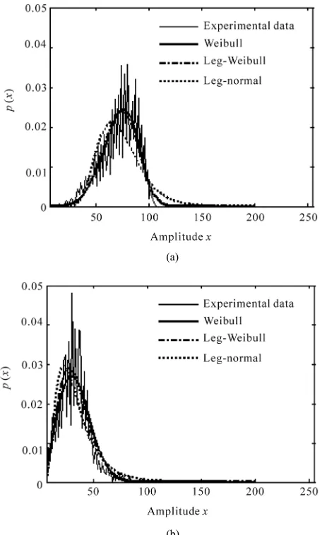
shown in Figure 4. The vertical axis is the probability,
and the horizontal axis shows the amplitude of the re-flected signal. The line-segment graph is the rere-flected- signal-amplitude observed data, and the curved lines are the probability density distributions. This confirms, even visually, that for ranges where there is no target the Wei- bull distribution corresponds better to the data regardless of whether the SWH is high or low.
4. Effect on the Reflected Amplitude
Distribution by Changes in the Sea
Surface
In order to investigate how changes in the state of the sea surface affect the statistical characteristics of sea clutter, we analyzed the correlation between the SWH and wave period and the parameters calculated from the distribu-tion estimadistribu-tion, for the 65 observadistribu-tion data sets under
(a)
[image:7.595.59.287.299.678.2](b)
Figure 4. Result of distribution estimation for range num-ber 6. (a) Significant wave height of 1.27 m; (b) Significant wave height of 0.21 m.
study and the range with no reflective objects other than waves (range no. n = 6).
4.1. Sea Surface Changes
Changes in the height and period of significant waves during the observation period are shown in Figure 5. The
horizontal axis shows the observation numbers assigned to each observation in order. The results show SWH ranging from 0.21 to 1.27 m and wave period ranging from 3.1 to 5.1 s.
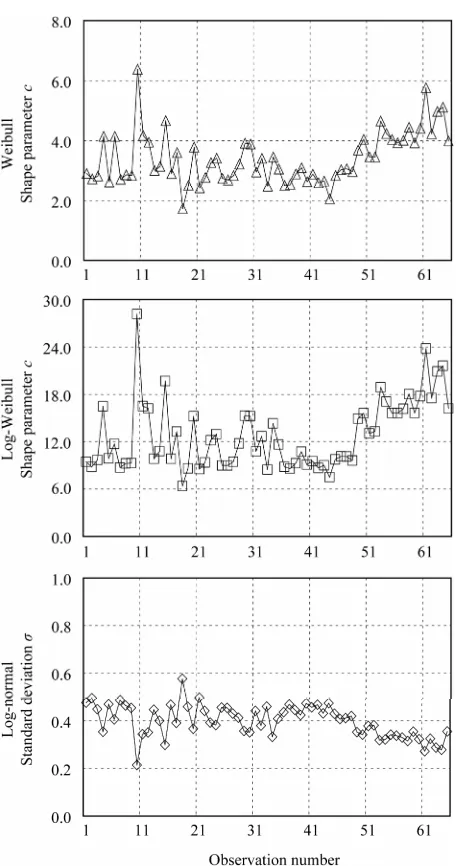
4.2. Sea Surface and Estimated Parameter Changes
How the parameters of each distribution changed as the state of the sea surface changed is shown in Figure 6.
The horizontal axis shows observation number, while the vertical axis shows the Weibull distribution shape pa-rameter, c, the Log-Weibull distribution shape papa-rameter, c, and the Log-normal distribution standard deviation, σ. As the state of the sea surface changed, the shape pa-rameter, c, of the Weibull distribution fluctuated between 1.74 and 6.38, that of the Log-Weibull between 6.38 and 28.17, and the standard deviation, σ, of the Log-normal distribution ranged from 0.214 to 0.576.
4.3. Relation between SWH and Estimated Parameters
The correlations between the SWH and the shape pa-rameter, c, for the Weibull distribution, which conformed better when the SWH was both high and low, and the Log-Weibull distribution, are shown in Figure 7. From
this we see that the shape parameter, c, for the Weibull distribution had a correlation coefficient of 0.755, and for Log-Weibull distribution it was 0.794, so the Log-Wei- bull distribution showed a stronger correlation.
[image:7.595.311.538.513.703.2]Figure 6. Variation of estimated distribution.
4.4. Relation between Wave Period and Estimated Parameters
The correlation between wave period and the shape pa-rameter, c, for the Weibull and Log-Weibull distributions are shown in Figure 8. The correlation coefficient for the
Weibull shape parameter, c, is 0.436, and for the Log- Weibull distribution it is 0.499, so both are only weakly correlated.
5. Conclusions
We made observations of the sea clutter using X-band radar and the state of the sea surface in the area of the Uraga Suido Traffic Route, where vessels enter and leave Tokyo Bay, including the Daini Kaiho Sea Fortress. We
[image:8.595.309.538.86.368.2]Figure 7. Correlation between significant wave height and estimated distribution.
[image:8.595.310.538.409.691.2]estimated the distribution of the sea clutter reflected am-plitudes using Weibull, Log-Weibull, Log-normal and K-distribution models. We then compared the results of estimating the distributions with the sea-surface state data and studied the effects of changes in sea state on the statistical characteristics of the sea clutter.
As a result, ranges not containing a target conformed better to the Weibull distribution regardless of SWH, but observed ranges containing a target conforming more to the Log-Weibull distribution when the SWH was high, and conformed to a Log-normal distributions when the SWH was low. Also, for observed ranges not containing a target, SWH and the shape parameter, c, of the Weibull distribution correlated with correlation coefficient of 0.755, and for the Log-Weibull distribution this figure was 0.794. The correlation between wave period and Weibull distri-bution shape parameter, c, had a coefficient of 0.436, and for the Log-Weibull distribution, the coefficient was 0.449, so both were only weakly correlated to wave pe-riod.
In the future, it will be necessary to study new thresh-old detection CFAR methods that detect targets more accurately by setting thresholds using the distribution estimation results we have studied, and also to examine the use of SWH and other approaches to setting thresh-olds.
REFERENCES
[1] International Meteorological Organization Resolution A.817 (19), “ECDIS Performance Standards,” 2000. [2] M. Sekine, “Radar Signal Processing Techniques,” The
Institute of Electronics, Information and Communication Engineers, Tokyo, 1991.
[3] M. L. Skolnik, “Introduction to Radar System,” McGraw- Hill, New York, 1982.
[4] J. Croney, “Clutter on Radar Displays,” Wireless Engi-neering, Vol. 33, 1956, pp. 83-96.
[5] M. Sekine, T. Musha, Y. Tomita, T. Hagisawa, T. Irabu, E. Kiuchi, “On Weibull-Distributed Weather Clutter,” IEEE Transactions on Aerospace and Electronic Systems, Vol. AES-15, No. 6, 1979, pp. 824-830.
doi:10.1109/TAES.1979.308767
[6] M. Sekine and Y. Mao, “Weibull Radar Clutter,” Peter Peregrinus Ltd., London, 1990.
[7] M. Sekine, T. Musha, Y. Tomita and T. Irabu, “Suppres-sion of Weibull-Distributed Clutters Using a Cell-Aver-aging LOG/CFAR Receiver,” IEEE Transactions on Aerospace and Electronic Systems, Vol. AES-14, No. 5, 1978, pp. 823-826. doi:10.1109/TAES.1978.308637 [8] M. Sekine, T. Musha, Y. Tomita, T. Hagisawa, T. Irabu
and E. Kiuchi, “Suppression of Weibull-Distributed Wea- ther Clutter,” Proceedings of IEEE International Radar Conference, New York, 1980, pp. 294-298.
[9] P. Z. Peebles Jr., “Radar Principles,” John Wiley and Sons Inc., New York, 1998.
[10] Ministry of Land, Infrastructure, Transport and Tourism of Japan, “NOWPHAS, Nationwide Ocean Wave Informa-tion Network for Ports and HArbourS,” 2010.
http://www.mlit.go.jp/kowan/nowphas/index.html [11] N. L. Johnson, S. Kotz and N. Balakrishnan,
“Distribu-tions in Statistics: Continuous Univariate Distribu“Distribu-tions,” Wiley Series in Probability and Mathematical Statistics, 2nd Edition, Vol. 1, 1994.
[12] S. Sayama, S. Ishii and M. Sekine, “Amplitude Statistics of Sea Clutter Observed by L-band Radar,” IEEE Trans-actions onFundamentals and Materials, Vol. 126, No. 6, 2006, pp. 426-429. doi:10.1541/ieejfms.126.426
[13] Y. Sakamoto, M. Ishiguro and G. Kitagawa, “Information Statistics,” Kyoritsu Syuppan Co., Ltd., Tokyo, 1983. [14] S. Kullback and R. A. Leibler, “On Information and