OF MAXIMUM LIKELIHOOD ESTIMATES
IN LOG-LINEAR MODELS
Serveh Sharifi Far, Michail Papathomas* and Ruth King
University of Edinburgh and *University of St Andrews
Abstract: Log-linear models are typically fitted to contingency table data to de-scribe and identify the relationship between different categorical variables. How-ever, the data may include observed zero cell entries. The presence of zero cell entries can have an adverse effect on the estimability of parameters, due to pa-rameter redundancy. We describe a general approach for determining whether a given log-linear model is parameter redundant for a pattern of observed zeros in the table, prior to fitting the model to the data. We derive the estimable param-eters or functions of paramparam-eters and also explain how to reduce the unidentifiable model to an identifiable one. Parameter redundant models have a flat ridge in their likelihood function. We further explain when this ridge imposes some ad-ditional parameter constraints on the model, which can lead to obtaining unique maximum likelihood estimates for parameters that otherwise would not have been estimable. In contrast to other frameworks, the proposed novel approach informs on those constraints, elucidating the model that is actually being fitted.
Key words and phrases: Contingency table, Extended maximum likelihood
mate, Identifiability, Parameter redundancy, Sampling zero.
1. Introduction
Observations from multiple categorical random variables can be cross-classified
according to the combinations of the variables’ levels. This type of data is
often displayed in a contingency table where each cell count is the number
of subjects with a given cross-classification. Log-linear models are typically
fitted to such tables and examples of their applications are given by Agresti
(2002), Bishop et al. (1975) and McCullagh & Nelder (1989).
Zero cell counts can have an adverse effect on the estimability of
log-linear model parameters. Zero entries are of two main types; structural and
sampling zeros. If the expectation and variance of a cell count are zero, then
the entry is a structural zero. A sampling zero is an observed zero entry to
a cell with positive expectation. In this manuscript, we examine how zero
cell entries influence the estimability of log-linear model parameters, and
this is addressed with respect to parameter redundancy.
A model is not identifiable if two different sets of parameter values
generate the same model for the data, which often happens when a model
is over-parametrised. This cause of non-identifiability is termed
model can be rearranged as a function of a smaller set of parameters, which
are themselves functions of the initial parameters. Parameter redundant
models have a flat ridge in their likelihood surface which precludes unique
maximum likelihood estimates for some of the parameters (Catchpole &
Morgan, 1997). For a log-linear parameter redundant model, often
unde-fined or large standard errors for nonestimable parameters are reported by
numerical optimisation methods. An overview of identifiability and
param-eter redundancy is given by Catchpole & Morgan (1997) and Catchpole
et al. (1998). Cole et al. (2010) provide several ecological examples on this
topic. Identifiability is crucial when exploring complex associations between
factors, as interaction terms quickly become nonestimable in the presence
of zero cell counts. The development of methods that identify the highest
level of interaction complexity, which can be explored for a given data set,
is therefore important.
We develop a method for the detection of parameter redundancy for
log-linear models in the presence of sampling zero observations. The estimable
parameters and combinations of parameters are derived, and it is shown
how a parameter redundant model can be reduced to a non-redundant one
which is also identifiable. We refer to the proposed method as the
corresponding cells are omitted from the modelling and analysis, since they
are associated with cross-classifications that cannot be observed.
A comprehensive study of log-linear models for contingency tables was
developed by Haberman (1973), who proved that maximum likelihood
es-timates of model parameters are unique when they exist, and provided a
necessary and sufficient condition for the existence of cell mean estimates
in the presence of zero cell entries. This was further studied by Brown
& Fuchs (1983) via considering and comparing iterative methods, and
by Lauritzen (1996) via a polyhedral and graphical model framework. A
polyhedral version of Haberman’s condition for the existence of the
max-imum likelihood estimator (MLE) is provided by Eriksson et al. (2006).
Estimability of parameters under a non-existent MLE, within the extended
exponential families, is studied by Fienberg & Rinaldo (2012a), and is
de-veloped to higher dimensional problems by Wang et al. (2016). We refer
to these developments collectively as the “Existence of the Maximum
Like-lihood Estimator” or EMLE framework. The method demonstrates that
some of the parameters cannot be estimated when the MLE does not exist.
However, an extended estimator, where some of the elements of the
esti-mated cell mean vector are zero, always exists (Eriksson et al., 2006). In
initial parameters.
We compare the proposed parameter redundancy approach with the
EMLE method. The reduced models obtained by the two methods may
differ in terms of their parametrisation, but the parameter redundancy
ap-proach provides a reparametrisation that retains the original interpretation
of the parameters. This is because this method provides estimable
param-eters and linear combinations of paramparam-eters instead of just the estimable
subset of the model’s initial parameters. The parameter redundancy
ap-proach also reveals additional constraints imposed by the likelihood function
on some parameter redundant models. Standard statistical software
pack-ages report parameter estimates for such a model without informing on the
additional implied constraints.
Section 1.1 introduces the necessary notation. Section 2 describes the
determination of a parameter redundant model and the proposed
adapta-tion to log-linear models. The idea is illustrated by examples and a study
on saturated log-linear models. We also show when additional constraints
enable us to determine unique ML estimates for additional parameters, thus
specifying the model that is in fact fitted to the sparse table. In Section
3, the EMLE framework is reviewed, and in Section 4, the two approaches
dis-cussion.
1.1 Log-linear models for contingency tables
Adopting the notation in Overstall & King (2014), let V = {V1, . . . , Vm}
denote a set of m categorical variables, where thejth variable haslj levels.
The corresponding contingency table has n = Qmj=1lj cells. Let y denote
ann×1 vector corresponding to the observed cell counts. Each element of
yis denoted byyi,i= (i1. . . im) such that 06ij 6lj−1 andj = 1, . . . , m.
Here, i, identifies the combination of variable levels that cross-classify the given cell. We define L as the set of all n cross-classifications, so that
L=⊗m
j=1[lj], in which [lj] ={0,1, . . . , lj−1}. Then, N = P
i∈Lyi denotes
the sum of all cell counts. The yis are assumed to be observations from
independent Poisson random variables, Yi, such that, µi = E(Yi). Let E
denote a set of subsets of V. By adapting the notation of Johndrow et al.
(2014), the log-linear model assumes the form,
mi = logµi= X
e∈E
θe(i), (1.1)
where θe(i) ∈ R denotes the main effect or the interaction among the variables in e corresponding to the levels in i. The summation is over all members of E, which could be the set of all subsets of the variables (for
a convention, θ corresponds to e = ∅, so that when the set E contains
e = ∅ there is an intercept θ in the model. To allow for the existence of
unique parameter estimates, corner point constraints are applied, so that
parameters that incorporate the lowest level of a variable are set to zero. To
clarify the notation, consider this minimal example. Assume two categorical
variables, V ={X, Y}, with l1 =l2 = 2 levels. Then, the number of cells
in the l1 ×l2 table is 4 and L = {00,10,01,11}. The set of subsets of V,
E ={∅,{X},{Y}} constructs the following independence log-linear model,
shown as model (X, Y),
m00 = logµ00 =θ, m10= logµ10=θ+θ1X,
m01 = logµ01 =θ+θY1, m11= logµ11=θ+θ1X +θY1.
Alternatively to (1.1), forpparameters, we can write,mn×1 = logµn×1 =
An×pθp×1, whereAis a full rank design matrix with elements{0,1}.
There-fore, this model can be written as below, in which the subscript indices of
parameters are removed because there are only two possible variable levels,
logµ00
logµ10
logµ01
logµ11 =
1 0 0 1 1 0 1 0 1 1 1 1
θ θX θY .
For a model fitted to an lm table (with m variables, each classified inl
setting a one-to-one correspondence between the elements ofLand integers,
i= 1, . . . , lm, as
i= (i1. . . im) = i1l0+i2l1+· · ·+im−1lm−2+imlm−1+ 1. (1.2)
Thus, for the mentioned example, elements in L = {00,10,01,11}
corre-spond to {1,2,3,4} respectively.
2. The Parameter Redundancy approach
2.1 The derivative method
Goodman (1974) first used a derivative approach to detect identifiability
in latent structure models and m-way contingency tables. The generic
approach for the exponential family of distributions that we summarize
here was presented by Catchpole & Morgan (1997) and Catchpole et al.
(1998), and was also developed independently by Chappell & Gunn (1998)
and Evans & Chappell (2000) for compartmental models.
The mean vector µ = E(Y) of observations from a distribution that belongs to the exponential family of distributions, is expressible as a
func-tion of parameters θ = (θ1, . . . , θp). The derivative matrix D(θ), which
has elements,
Dsi(θ) =
∂µi
∂θs
, s = 1, . . . , p, i= 1, . . . , n. (2.3)
Theorem 1 of Catchpole & Morgan (1997) states that the model which
relatesµtoθ is parameter redundant if and only if the derivative matrix is
symbolically rank deficient. That is if there exists a non-zero vector α(θ)
such that for all θ,
α(θ)TD(θ) = 0. (2.4)
As an alternative, Cole et al. (2010) construct a derivative matrix by
differ-entiating an “exhaustive summary” of the model. An exhaustive summary
is a vector of parameter combinations that uniquely defines the model.
The rank of the derivative matrix, r, is the number of estimable
param-eters and combinations of paramparam-eters. The model deficiency is defined as
d=p−r, which is the number of linearly independentα(θ) vectors, labelled
asαj(θ), j = 1, . . . , d. Any elements of these vectors which are zero for all
j, correspond to the parameters that are directly estimable (Catchpole et
al., 1998). To find the estimable combinations of parameters, the auxiliary
equations of the following system of linear first order partial differential
equations need to be solved,
p X
s=1
αsj
∂f ∂θs
(Catchpole et al., 1998). The solution can be obtained using software such
asMaple which allows symbolic computations.
2.2 Parameter redundancy for log-linear models
Parameter redundancy occurs due to the model structure or lack of data
(Catchpole & Morgan, 2001; Cole et al., 2010), and the latter type is referred
to as “extrinsic” parameter redundancy (Gimenez et al., 2004). Model (1.1)
is constructed so that it is not over-parametrised due to its structure. To
detect extrinsic parameter redundancy for a log-linear model, we adjust the
derivative matrix elements (2.3) using yilogµi as a monotonic function of
µi, such that,
Dsi =
∂yilogµi
∂θs
, s= 1, . . . , p, i= 1, . . . , n. (2.6)
In effect, each sampling zero turns a column of the derivative matrix to zero
and may decrease the rank of the derivative matrix.
If the rank of the derivative matrix is smaller than p, the model is
pa-rameter redundant. Finding all estimable papa-rameters and estimable
combi-nations of parameters further identifies which cell means are estimable. The
vector of estimable quantities (θ0) and the vector of estimable cell means
(µ0) specify a reduced model via a smaller design matrix (A0). The reduced
estimable cell means minusr.
To clarify the notation, consider the independence log-linear model
(X, Y) for a 2 × 2 table. The derivative matrix (2.6) for observations
yT = (y
1, y2, y3, y4) = (y00, y10, y01, y11) and parameters θT = (θ, θX, θY)
is,
D=
∂yilogµi
∂θs
=
µ00 µ10 µ01 µ11
θ y1 y2 y3 y4
θX 0 y2 0 y4
θY 0 0 y3 y4
, s= 1,2,3, i= 1,2,3,4.
Now, for example, assume that y1 =y2 = 0. Then,r = 2, d= 1 andαT=
(1,0,−1). Equation (2.5) is ∂f∂θ −∂θ∂fY = 0 and solving it gives the estimable
parametersθ0T= (θX, θ+θY). It determines that onlyµ0T = (µ01, µ11) are
estimable. Therefore, the reduced design matrix A0 is 2×2 with two rows
[(0,1),(1,1)].
Alternative approaches for investigating identifiability are not suitable
in the context of Poisson log-linear models for contingency tables.
Specifi-cally, using the log-likelihood function elements as exhaustive summaries is
a common option in forming the derivative matrix (Cole et al., 2010).
Sim-ilarly, Catchpole & Morgan (2001) use the score vector of a multinomial
log-linear model to assess the effect of missing data on the model
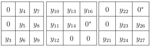
Table 1: Observations in a 33 contingency table
0 y4 y7
0 y5 y8
y3 y6 y9
y10 y13 y16
y11 y14 0∗
y12 0 0
0 y22 0∗
0 y23 y26
y21 y24 y27
is an alternative for detecting non-identifiability (Rothenberg, 1971).
How-ever, these approaches do not necessarily show the rank deficiency caused by
the zero cell counts for a Poisson log-linear model. The next two examples
further illustrate the use of the parameter redundancy method.
Example 1. The data pattern in Table 1, taken from Fienberg & Rinaldo (2012a), describes cell counts for variables X (rows), Y (columns), and Z
(layers), with three levels (0,1,2) for each. Eight cell counts are observed
as sampling zeros. All other cell counts are positive Poisson observations,
numbered according to (1.2). We fit the hierarchical model (XY, XZ, Y Z)
which can be shown as logµ27×1 =A27×19θ19×1,with parameters,
θT= (θ, θX1 , θ2X, θY1, θ2Y, θ1Z, θZ2, θ11XY, θ21XY, θ12XY, θXY22 ,
θ11Y Z, θY Z21 , θY Z12 , θY Z22 , θXZ11 , θXZ21 , θXZ12 , θ22XZ).
The matrix form of this model is given in the Supplementary Material.
there are only 18 estimable parameters or combinations of them. So, d =
19−18 = 1, and the αthat satisfies (2.4) is,αT= (1,0,−1,−1,−1,−1,0,
0,1,0,1,1,1,0,0,0,1,0,0).Solving (2.5) gives the estimable quantities as,
θ0T= (θ1X, θ+θ2X, θ+θY1, θ+θY2, θ+θZ1, θ2Z, θXY11 ,−θ+θ21XY, θXY12 ,−θ+θ22XY,
−θ+θ11Y Z,−θ+θ21Y Z, θ12Y Z, θ22Y Z, θ11XZ,−θ+θ21XZ, θXZ12 , θXZ22 ).
The elements of θ0 determine that 21 out of 27 cell means are estimable,
including cells 17 and 25, indicated in Table 1 with asterisks. Therefore, for
this model and this specified pattern of zeros, cell means 1,2,15,18,19,20
are not estimable. As these cell means are not estimable, we remove the
corresponding cells from the model. This is equivalent to assuming that
those observations are structural zeros. Consideringθ0 and the 21 estimable
cell means, the reduced model with three degrees of freedom is logµ021×1 =
A021×18θ180 ×1, given in the Supplementary Material.
Example 2. Hung et al. (2008) performed a genome-wide association study of lung cancer by studying 500 Single Nucleotide Polymorphisms (SNP).
Each SNP is categorized at levels 0, 1 and 2 to identify the number of
mi-nor alleles. Papathomas et al. (2012) selected 50 of these SNPs via applying
profile regression. We further select five SNPs (as representatives of
(C),rs11128775_G (D),rs9306859_A (E).
A crucial variable in this study describes the presence or absence of
cancer in each of the individuals. Adding this variable (F) creates a 35×21
contingency table with 486 cells. We consider fitting a log-linear model with
main effects and first-order interactions. This table has 298 zero cell counts
and the derivative matrix has rank 59 withd = 62−59 = 3. After solving
the partial differential equations for the three α vectors, the 59 estimable
parameters are obtained and given in the Supplementary Material.
Only three parameters θAD
22 , θAE22 , θ22DE are not estimable. The estimable
parameters make 360 out of 486 cell means estimable and the reduced model
is, logµ0360×1 = A0360×59θ590 ×1, with degrees of freedom 360−59 = 301. In
this model, the presence of cancer has a significant positive interaction with
level 1 of variablesAandDand a significant negative interaction with level
1 of C and E and level 2 of B, C and E.
2.3 Parameter redundancy for a saturated log-linear model
We provide some general results on parameter redundancy for a saturated
log-linear model fitted to an lm contingency table and determine which
parameters become nonestimable after observing a zero cell count. Example
shows that a saturated log-linear model is always full rank when all the cell
counts are positive.
Definition 1. For a saturated log-linear model, we define the parameter corresponding to the cell with count yi, i= 1, . . . , n (according to (1.2)), as
the one with the maximum number of variables in its superscript, within
the set of all parameters in logµi =A(i)θ, whereA(i) is the ith row of A.
For example, for a 33 contingency table with variables {X, Y, Z}, the
pa-rameter corresponding to observation y201 (or y12according to the ordering
given by (1.2)) is θXZ 21 .
Definition 2. For a given log-linear model parameter, parameters asso-ciated with a higher order interaction are all those specified by including
additional variables in the given parameter’s superscript.
For example, for the same 33 table, the parameters associated with a higher
order interaction given θXZ
21 , are θ211XY Z and θXY Z221 .
The following theorem determines exactly which model parameters
be-come nonestimable as a result of a given zero observation.
Theorem 1. Assume a saturated Poisson log-linear model fitted to an lm
parameter that corresponds to that cell, and all other parameters associated
with a higher order interaction given that parameter, are nonestimable.
The proof by induction and examples are given in the Supplementary
Ma-terial. Note that additional zero cells in the table cannot make previously
nonestimable parameters estimable, as the amount of information is
fur-ther reduced. Then, the set of nonestimable parameters is at least as large
as the union of the nonestimable parameters per zero cell. The estimable
parameters and linear combinations of them can be derived by solving (2.5).
2.4 The esoteric constraints
The likelihood function of parameter redundant models has a flat ridge
which is occasionally orthogonal to the axes of some parameters, so these
associated parameters still have unique ML estimates (Catchpole et al.,
1998). This is when in all α(θ)s, the corresponding elements to these
pa-rameters are zero. In addition, for some log-linear parameter redundant
models, maximising the likelihood function imposes one or more extra
con-straints on the model parameters, due to the placement of the likelihood
ridge in the parameter space. The extra constraints can make more
param-eters uniquely estimable compared to those specified by solving the partial
“es-oteric constraints”. Standard statistical software packages do not provide
any information on these constraints when maximising the likelihood
func-tion, so informing on them reveals the log-linear model that is, in fact,
being fitted. After detecting a parameter redundant model, we can check
the existence of such constraints, as explained below.
The log-likelihood function of model (1.1) is l(θ) = P
i(yilogµi(θ)−
µi(θ)). The corresponding score vector is U(θ) = (∂l/∂θ1,· · · , ∂l/∂θp)T,
where the partial derivatives for s= 1, . . . , p, are,
∂l ∂θs
=X
i
yi
µi(θ)
−1
∂µi(θ)
∂θs
=X
i
(yi−µi(θ))
∂µi(θ)
∂θs
1 µi(θ)
.
Therefore, U(θ) = AT(y−µ(θ)). When a model is parameter redundant, there exists at least oneα(θ) such thatαT(θ)D(θ) =0. If the observations are from a multinomial distribution, it follows that αT(θ)U(θ) = 0, which means the likelihood surface has a completely flat ridge (Theorem 2 of
Catchpole & Morgan (1997)). Note that, αT(θ)U(θ) = 0 implies that the directional derivative is zero, therefore, the likelihood function is constant
in the direction ofα(θ). This makes a ridge in the likelihood surface, which
is along the curve generated by the direction field α(θ) through any point
at which the likelihood is maximised.
For a Poisson log-linear model which is determined to be parameter
constraints that hold this equality for finite values of the model
parame-ters, are the esoteric constraints. These extra constraints along with the
estimable quantities in θ0, may make more parameters estimable and
per-mit one to obtain unique maximum likelihood estimates for parameters
that otherwise would not have been estimable. Also, reducing the
param-eter space according to the esoteric constraints and therefore removing the
flat ridge, can make it possible to uniquely maximise the likelihood. If
αT(θ)U(θ) cannot be zero with finite θs then the esoteric constraints do not exist and some of theθs tend to negative infinity. These constraints do
not exist for models described in Theorem 1 and in Examples 1 and 2. A
model with an esoteric constraint is given in Example 4.
3. The existence of the maximum likelihood estimator for log-linear models
The methods summarized in this section will be referred to as the EMLE
approach and will be used in Examples 3 and 4 in Section 4. We refer the
reader to Fienberg & Rinaldo (2006, 2012a,b) for further background and
details.
Decomposable log-linear models (Agresti, 2002) have an explicit
is a necessary and sufficient condition for the existence of the MLE of µ
(Agresti, 2002). For non-decomposable models, ˆµi does not have a closed
form and it is calculated only by iterative methods. In this case,
positiv-ity of sufficient table marginals is still necessary for the existence of the
estimator but it is no longer a sufficient condition.
A condition for the existence of the MLE of m in a hierarchical log-linear model, regardless of the presence of positive or zero table marginals,
was provided by Haberman (1973). Assume M is a p-dimensional linear
manifold contained in R|L|, and
M⊥=
x∈ R|L|
: (x,m) =xTm= 0,∀m∈ M . (3.7)
Then, Theorem 3.2 of Haberman (1973) states that a necessary and
suf-ficient condition that the MLE ˆm of m exists is that there is a δ ∈ M⊥ such that yi+δi > 0 for every i ∈ L. Here, µ in m = logµ is assumed
to be positive. The theorem specifies, for any pattern of zeros in the table,
whether the MLE of the cell means exists or not. In the extended maximum
likelihood estimate case, a cell mean estimate could be ˆµi = 0, but its log
transformation is not defined and then estimates of some corresponding θ
parameters tend to infinity (Haberman, 1974).
A polyhedral version of Haberman’s necessary and sufficient condition
the vector of observed marginals, t = ATy, lies in the relative interior of the marginal of the polyhedral cone (Eriksson et al., 2006). The polyhedral
cone, generated by spanning columns of A with rankp, is defined as,
CA={t:t=ATy,y∈ R
|L|
>0}. (3.8)
The MLE does not exist if and only if the vector of marginals lies on a facet
or a facial set of the marginal cone (Fienberg & Rinaldo, 2006). In other
words, the estimator does not exist if and only if the vector of marginals
belongs to the relative interior of some proper face,F, of the marginal cone.
A face of the marginal cone is defined as a set, F = {t∈CA : (t,ζ) = 0},
for someζ ∈ Rp, such that (t,ζ)>0 for allt∈C
A, with (t,ζ) representing
the inner product. The facial set F is a set of cell indices of the rows of A
whose conic hull is preciselyF. For any design matrix A for M, F ⊆L is
a facial set ofF if there exists someζ ∈ Rp such that,
(A(i),ζ) = 0, if i∈ F, (3.9)
(A(i),ζ)>0, if i∈ Fc,
where Fc = L− F is the co-facial set of F (Fienberg & Rinaldo, 2012a).
If such ζ and F exist, the MLE does not exist and only the cell means
corresponding to members of F are estimable. The nonestimable cells in
estimable subset of model parameters could be determined by finding AF,
the matrix whose rows are the ones fromAwith coordinates inF. AF which
is a |F | ×p design matrix with rank pF, is then reduced to full rank A∗F
with dimensions|F | ×pF. By implementing this reduced design matrix, the
log-likelihood function is strictly concave with a unique maximiser. Then
the extended MLE is,
ˆ
θe = argmaxθ∈RpFlF(θ) = argmaxθ∈RpFtTFθ−1
T
exp(A∗Fθ),
in which tF = (A∗F)TyF and the extended MLE of the cell mean vector is ˆ
me= exp(A∗Fθˆe) (Fienberg & Rinaldo, 2012b).
Another way to define the facial set is by considering sub-matrices A+
and A0 obtained from A. They are made by the rows of A indexed by
L+ = {i : yi 6= 0} and L0 = {i : yi = 0} respectively. The vector of
marginals belongs to the relative interior of some proper face of the marginal
cone if and only if Fc⊆L
0. This is equivalent to the existence of a vector ζ satisfying the following three conditions (Fienberg & Rinaldo, 2012b):
a. A+ζ =0, (3.10)
b. A0ζ 0,
c. The set{i: (Aζ)(i)6= 0}has maximal cardinality among all sets of
In (3.9) and (3.10) the inequality signs could be changed to less than zero
without loss of generality. With 0 we describe a non-negative vector
with at least one element greater than zero. In conclusion, if rank(A+) =
rank(A), the MLE exists, since no vectorζexists andFc =∅. If rank(A +)<
rank(A), the MLE may still exist, so we should search for a facial set.
The degrees of freedom for the reduced model is|F |−rank(A∗F), which is
the number of estimable cell means minus the number of estimable model
parameters (Fienberg & Rinaldo, 2012a). Computational algorithms for
detecting the existence of the MLE and deriving the co-facial set, by
con-verting these methods into linear and non-linear optimisation problems, are
described by Fienberg & Rinaldo (2012b). However, those algorithms are
inefficient for a model with a large number of variables (Wang et al., 2016).
The Rpackages eMLEloglin and SparseMSEutilize the EMLE approach to
fit log-linear models (Chan et al., 2019; Friedlander, 2016).
4. Comparison of the EMLE and the parameter redundancy ap-proaches
The two approaches described in Sections 2 and 3 can be used to check the
identifiability of a log-linear model fitted to a sparse table. We compare
i. Within the EMLE framework, when the co-facial set, as defined in
(3.9), is null, then the MLE exists. This is equivalent to the parameter
redundancy outcome in which the model is not parameter redundant.
ii. When there are facial and co-facial sets as defined in (3.9), the MLE
ofµdoes not exist and some zero cells are treated as structural zeros.
In the parameter redundancy approach, this is equivalent to having
αTD=0and no esoteric constraints determined by αTU(θ) = 0. In practice, for such a model, the determinant of the information matrix
and at least one of its eigenvalues are very close to zero, considering
numerical approximations and rounding errors.
iii. If there is no co-facial set as described in (3.9), then the MLE exists.
This is equivalent to the parameter redundancy outcome in which the
model is parameter redundant with at least one esoteric constraint
that allows one to uniquely estimate the model parameters.
The next theorem explains a link between the EMLE method and the
pa-rameter redundancy approach through the score vector U(θ).
Theorem 2. For a parameter redundant model, the MLE of µ does not exist if and only if one or more αj vectors, j = 1, . . . , d, do not satisfy
αT
The proof is given in the Appendix.
Two examples are utilized here to illustrate similarities and differences
between the two approaches. Example 3 below shows a parameter
redun-dant model without any possible additional esoteric constraints (comparison
case ii). The two reduced models found by the two approaches have a
dif-ferent reparametrisation of θ, although the ML estimates of the estimable
cell means are identical. The parameters in the reduced model obtained
by parameter redundancy have the same interpretation as in the initial
model, in terms of variable interactions. Example 4 presents a model that
is parameter redundant and its MLE does exist (comparison case iii). This
model has an esoteric constraint, extracted by the parameter redundancy
approach, that makes all parameters estimable. This approach allows us to
consider two possible ways to address the model’s redundancy. Reduce the
model to a smaller, saturated and non-redundant one, or adopt the esoteric
constraint and estimate all parameters, which is equivalent to using
numer-ical methods such as “iteratively reweighted least squares” to maximise the
likelihood.
Example 3. We fit model (4.11), which can be shown as (XY, XZ, Y Z), to the contingency table in Table 2(a).
logµijk =θ+θiX+θ Y j +θ
Z k +θ
XY ij +θ
XZ ik +θ
Y Z
jk , i, j, k ={0,1}
Table 2: Observations in two 23 contingency tables
(a)
Z = 0 Z = 1
Y = 0 Y = 1 Y = 0 Y = 1
X= 0 0 y3 y5 y7
X= 1 y2 y4 y6 0
(b)
Z = 0 Z = 1
Y = 0 Y = 1 Y = 0 Y = 1
X = 0 0 y3 y5 y7
X = 1 y2 0 y6 y8
According to (1.2), the vector of cell counts isyT = (y
1, y2, y3, y4, y5, y6, y7, y8)
= (y000, y100, y010, y110, y001, y101, y011, y111). The non-zero cell counts in the
table are assumed to be positive. The parameter vector is shown as θT =
(θ, θX, θY, θXY, θZ, θXZ, θY Z) as subscripts are superfluous. The model in
the form logµ8×1 =A8×7θ7×1 is given in the Supplementary Material.
We apply the parameter redundancy approach first. The derivative
ma-trix formed using formula (2.6) is given in the Supplementary Material and
its rank is 6, indicating that d= 1. From (2.4), αT= (1,−1,−1,1,−1,1,
1) and solving (2.5) yields the estimable parameters,
θ0T= (θ+θX, θ+θY,−θ+θXY, θ+θZ,−θ+θXZ,−θ+θY Z).
Therefore, all cell means but µ000 (for which, logµ000 = θ) and µ111 (for
which, logµ111 =θ+θX +θY +θXY +θZ+θXZ+θY Z) are estimable. No
esoteric constraint exists as,
αTU(θ) = y000+y111−eθ−eθ+θ
X+θY+θXY+θZ+θXZ+θY Z
6
for finite θs. We treat y000 and y111 as structural zeros and remove them
from the model. Then, we reduce the model to a saturated one with a
design matrix of rank 6 in accordance with the estimable parameters θ0.
The reduced non-redundant model is,
logµ100
logµ010
logµ110
logµ001
logµ101
logµ011 =
1 0 0 0 0 0
0 1 0 0 0 0
1 1 1 0 0 0
0 0 0 1 0 0
1 0 0 1 1 0
0 1 0 1 0 1
θ+θX θ+θY
−θ+θXY
θ+θZ
−θ+θXZ
−θ+θY Z
.
Now we consider the EMLE method. Model (4.11) has no zero sufficient
marginals, but positive estimates for all the cell means do not exist
accord-ing to the Haberman’s sufficiency and necessary condition and also the
poly-hedral condition. To reduce this model to an identifiable one, according to
the polyhedral method and (3.9), we obtain, F ={100,010,110,001,101,
011}, Fc ={000,111}, and ζ = (1,−1,−1,1,−1,1,1). The design matrix
for the reduced model isA∗F, which is a|F |×pF = 6×6 matrix and is found
by using the suggested Proposition 5.1 in Fienberg & Rinaldo (2012b). The
final model is,
logµ100
logµ010
logµ110
logµ001
logµ101
logµ011 =
1 1 0 0 0 0
1 0 1 0 0 0
1 1 1 1 0 0
1 0 0 0 1 0
1 1 0 0 1 1
1 0 1 0 1 0
The estimable cell means are the same as derived by the parameter
redun-dancy approach (as must be the case). However, θY Z is dropped from the
model reducing it to (XY, XZ).
In a numerical example, the ML estimates for the six estimable cell
means are identical under the two methods and log-linear model parameter
estimates are also consistent. Although both methods reduce the model to
one with six parameters, parameter interpretations differ. The parameters
derived by the parameter redundancy approach are the linear combinations
of the ones in the initial model. However, for instance, the estimate ofθ in
the second reduced model is not the intercept estimate for the initial model.
Example 4. Consider fitting model (4.11) to the pattern of zeros in Table 2(b). For the parameter redundancy approach, the derivative matrix is
given in the Supplementary Material and its rank is 6, thus d = 1. Then,
αT= (1,−1,−1,0,−1,1,1) indicates the estimable parameters as,
θ0T= (θ+θX, θ+θY, θXY, θ+θZ,−θ+θXZ,−θ+θY Z).
Therefore, logµ000 and logµ110 are not estimable. The initial model is
logµ100
logµ010
logµ001
logµ101
logµ011
logµ111 =
1 0 0 0 0 0
0 1 0 0 0 0
0 0 0 1 0 0
1 0 0 1 1 0
0 1 0 1 0 1
1 1 1 1 1 1
θ+θX θ+θY θXY θ+θZ
−θ+θXZ
−θ+θY Z
.
However, an esoteric constraint exists and it is derived by considering,
αTU(θ) =y000−y110−eθ+eθ+θ
X+θY+θXY
= 0.
This translates to θX +θY +θXY = 0 or logµ
000 = logµ110. Adding this
constraint on model (4.11) makes all parameters estimable.
In accordance with the EMLE approach for model (4.11), we identify
a δ which satisfies (3.7), such that yi +δi > 0,∀i ∈ L. Let 0 < δ < 1,
thenδ = (+δ,−δ,−δ,+δ,−δ,+δ,+δ,−δ) holds the necessary and sufficient
condition for the existence of the estimator of µ. This is also confirmed
by the polyhedral condition since the observed marginals lie in the relative
interior of the marginal of the polyhedral cone, as vector y = (y1+δ, y2−
δ, y3−δ, y4+δ, y5−δ, y6+δ, y7+δ, y8−δ) satisfies (3.8). In other words, noζ
orFcan satisfy (3.9) or (3.10). Thus, we are able to maximise the likelihood
function by numerical methods and obtain the estimates for all parameters
of model (4.11). This is possible because of the esoteric constraint, which
is not reported by this method but is explicit in the parameter redundancy
5. Discussion
We propose a parameter redundancy approach for evaluating the effect of
zero cell counts on the estimability of log-linear model parameters. For
a parameter redundant model, we obtain the estimable parameters and
reduce the model to an identifiable one.
We compare the parameter redundancy approach with a different method
that focuses on the existence of the MLE for the expected cell counts of a
hierarchical model. Models with non-existent MLE are parameter
redun-dant, whilst some log-linear models are parameter redundant despite their
existent MLE. The latter happens when maximising the likelihood function
which has a flat ridge, imposes hidden extra constraints on the model to
make a unique MLE possible.
The EMLE method is reported by Wang et al. (2016) to be inefficient
in finding the co-facial sets when the number of variables in the model is
larger than 16. The authors propose an approximation for the cone’s face to
make the method work for more variables. In the parameter redundancy
ap-proach, the symbolic algebra packageMaple can be used to simultaneously
solve a number of corresponding partial differential equations. However,
as Maple runs out of memory, problems arise in the calculations when the
this limitation depends on the fitted model and the pattern of zeros in the
table. For example, it may become more notable in applications such as
large cohort studies, when observations are concentrated in a small subspace
of the entire sample space.
Future research could further explore the parameter redundant models
with existent MLE. This includes further investigating properties of the
esoteric constraints and goodness of fit of the model implied by them.
Supplementary Material
The online Supplementary Material contains more details of some of
the examples, Example S1, and proof of Theorem 1 by induction.
Acknowledgments
We would like to thank the referees and the journal editor for comments
that improved this manuscript. The work of first author is supported by
EPSRC PhD grants EP/J500549/1, EP/K503162/1 and EP/L505079/1.
Appendix
Proof of Theorem 2. Assume the MLE does not exist for a parameter
redundant model. We prove by contradiction that at least one αj vector
does not satisfy αT
αj vectors, j = 1, . . . , d, satisfy αjT(θ)U(θ) = 0 for finite elements of θ.
We know U(θ) =AT(y−µ(θ)). Then,
αT
j(θ)U(θ) = 0 αTjAT(y−µ(θ)) = 0,
αT
jAT+(y−µ(θ))++αTjAT0(y−µ(θ))0 = 0,
where (y−µ(θ))+ denotes a vector with the elements of (y−µ(θ)) that
correspond to the rows in A+, and (y − µ(θ))0 denotes a vector with
the elements of (y − µ(θ)) that correspond to the rows in A0. Now,
αTjAT+(y−µ(θ))+ = 0, because αTjAT+ = 0, since αTjD = 0. This
im-plies that αTjAT0(y−µ(θ))0 = 0, or equivalently that αTjAT0(−µ(θ))0 = 0.
As the MLE does not exist, from (3.10), aζ vector exists so that A0ζ 0.
However, ζ is also an α vector, as A+ζ = 0. Now suppose, without any
loss of generality, that αj0 =ζ, 16j 0
6d. Then,
A0αj0 0 ⇒ α
T
j0A
T
0(−µ(θ))0 <0,
as all elements of (−µ(θ))0 are non-zero and negative. Thus, this
contra-dicts αT
jAT0(−µ(θ))0 = 0.
αT
j(θ)U(θ)<0 and cannot be zero for finite θ. This implies that,
αTjAT+(y−µ(θ))++αTjA
T
0(y−µ(θ))0 <0,
αTjAT0(−µ(θ))0 <0,
since αT
jD=0 means αTjAT+=0. Thus, αTjAT0 0. From all αj’s so that αT
jAT0 0, we choose the αj0 that corresponds to the set {i: (Ax)(i)6= 0}
with maximal cardinality. Then,αj0 satisfies the three conditions in (3.10),
and the MLE does not exist. This completes the proof of Theorem 2.
References
Agresti, A. (2002). Categorical Data Analysis. Second Edition. Wiley, New York.
Bishop, Y. M. M., Fienberg, S. E. and Holland, P. W. (1975). Discrete Multivariate Analysis, Theory and Practice. The MIT Press.
Brown, M. B. and Fuchs, C. (1983). On Maximum likelihood estimation in sparse contingency tables. Computational Statistics and Data Analysis,1, 3–15.
Catchpole, E. A. and Morgan, B. J. T. (1997). Detecting parameter redundancy. Biometrika,
84, 187–196.
Catchpole, E. A. and Morgan, B. J. T. (2001). Deficiency of parameter redundant models.
Biometrika,88(2), 593–598.
Chan, L., Silverman, B. and Vincent, K. (2019).Multiple Systems Estimation for Sparse Capture Data: Inferential Challenges when there are Non-Overlapping Lists. arXiv:1902.05156v1. Chappell, M. J. and Gunn, R. N. (1998).A procedure for generating locally identifiable
reparam-eterisations of unidentifiable non-linear systems by the similarity transformation approach.
Mathematical Biosciences,148(1), 21–41.
Cole, D. J., Morgan, B. J. T. and Titterington, D. M. (2010).Detecting the parametric structure of models. Mathematical Biosciences,228, 16–30.
Eriksson, N., Fienberg, S. E., Rinaldo, A. and Sullivant, S. (2006). Polyderal conditions for the nonexistence of the MLE for hierarchical log-linear models. Journal of Symbolic Compu-tation,41, 222–233.
Evans, N. D. and Chappell, M. J. (2000). Extensions to a procedure for generating locally iden-tifiable reparameterisations of unideniden-tifiable systems. Mathematical Biosciences, 168(2), 137–159.
Fienberg, S. E. and Rinaldo, A. (2006).Computing maximum likelihood estimation in log-linear models. Carnegie Mellon University.http://www.stat.cmu.edu/tr/tr835/tr835.pdf
Fienberg, S. E. and Rinaldo, A. (2012a). Maximum likelihood estimation in log-linear models.
Fienberg, S. E. and Rinaldo, A. (2012b). Maximum likelihood estimation in log-linear models, Supplementary material: Algorithms.
http://www.stat.cmu.edu/~arinaldo/Fienberg_Rinaldo_Supplementary_Material.pdf.
Friedlander, M. (2016). Fitting log-linear models in sparse contingency tables using the eMLEl-oglin R package. arXiv:1611.07505.
Gimenez, O., Viallefont, A., Catchpole, E. A., Choquet, R. and Morgan, B. J. T. (2004).
Methods for investigating parameter redundancy. Animal Biodiversity and Conservation,
27, 1–12.
Goodman, L. A. (1974).Exploratory latent structure analysis using both identifiable and uniden-tifiable models. Biometrika,61(2), 215–231.
Haberman, S. J. (1973).Log-linear models for frequency data: Sufficient statistics and likelihood equations. The Annals of Statistics,1(4), 617–632.
Haberman, S. J. (1974).The Analysis of Frequency Data. University of Chicago press, Chicago. Hung, R.J. et al. (2008). A susceptibility locus for lung cancer maps to nicotinic acetylcholine
receptor subunit genes on 15q25. Nature,452, 633-637.
Johndrow, J. E., Bhattacharya, A.l. and Dunson, D. (2017). Tensor decompositions and sparse log-linear models. The Annals of Statistics,45(1), 1-38.
McCullagh, P. and Nelder, J. A. (1989). Generalized linear models. Second Edition, Chapman and Hall, London.
Overstall, A. M. and King, R. (2014).conting: An R package for Bayesian analysis of complete and incomplete contingency tables. Journal of Statistical Software,58(7), 1–26.
Papathomas, M., Molitor, J., Hoggart, C., Hastie, D. and Richardson, S. (2012). Exploring data from genetic association studies using Bayesian variable selection and the Dirichlet
process: Application to searching for gene × gene patterns. Genetic Epidemiology, 36, 663–674.
Rothenberg, T. J. (1971).Identification in parametric models. Econometrica,39(3), 577–591. Wang, N., Rauhyand, J. and Massam, H. (2019). Approximating faces of marginal polytopes in
discrete hierarchical models. The Annals of Statistics,47(3), 1203–1233.
Department of Statistics, School of Mathematics, University of Edinburgh, EH9 3FD, UK. E-mail: [email protected]
Department of Statistics, School of Mathematics and Statistics, University of St Andrews, KY16 9LZ, UK. E-mail: [email protected]