Statistical modelling of individual animal movement: an
overview of key methods and a discussion of practical challenges
Toby A. Patterson
CSIRO Oceans and Atmosphere, Hobart, Australia
[email protected]
Alison Parton
School of Mathematics and Statistics, University of Sheffield, UK
[email protected]
Roland Langrock
Department of Business Administration and Economics, Bielefeld University, Germany
[email protected]
Paul G. Blackwell
School of Mathematics and Statistics, University of Sheffield, UK
[email protected]
Len Thomas
School of Mathematics and Statistics, University of St Andrews, UK
[email protected]
Ruth King
School of Mathematics, University of Edinburgh, UK
[email protected]
Abstract
With the influx of complex and detailed tracking data gathered from electronic tracking
de-vices, the analysis of animal movement data has recently emerged as a cottage industry amongst
biostatisticians. New approaches of ever greater complexity are continue to be added to the
liter-ature. In this paper, we review what we believe to be some of the most popular and most useful
classes of statistical models used to analyze individual animal movement data. Specifically we
con-sider discrete-time hidden Markov models, more general state-space models and diffusion processes.
We argue that these models should be core components in the toolbox for quantitative researchers
working on stochastic modelling of individual animal movement. The paper concludes by offering
some general observations on the direction of statistical analysis of animal movement. There is a
are inaccessible to ecologists, unwieldy with large data sets or not based in mainstream statistical
practice. Additionally, some analysis methods developed within the ecological community ignore
fundamental properties of movement data, potentially leading to misleading conclusions about
an-imal movement. Corresponding approaches, e.g. based on L´evy walk-type models, continue to be
popular despite having been largely discredited. We contend that there is a need for an appropriate
balance between the extremes of either being overly complex or being overly simplistic, whereby
the discipline relies on models of intermediate complexity that are usable by general ecologists, but
grounded in well-developed statistical practice and efficient to fit to large data sets.
Keywords: hidden Markov model; measurement error; Ornstein-Uhlenbeck process; state-space model;
stochastic differential equation; time series
1
Introduction
Movement ecology seeks to infer why organisms move through space and what constraints operate on
them as they do. It is the study of how movement shapes their overall ecology, and the factors, both
intrinsic and extrinsic, that influence movement. Movement ecology broadly concerns the study of
both animals and plant movement and dispersal. While there are commonalities in some aspects of
their study, there are also many differences. In this paper we concern ourselves purely with individual
organismal movement as measured through instruments and sensors which record position at relatively
short time scales. Although it is possible that some of the aspects we discuss also apply to plants,
practically this means we are nearly always referring to the study of animal movement.
The discipline has been driven by the possibility of telemetering the paths of free-moving animals
navigating their natural habitats. Devices such as satellite and GPS tags, radio tracking, radar and
acoustic monitoring have generated large and, to ecologists and statisticians alike, largely unfamiliar data
sets. Each technology has its limitations and strengths in terms of accuracy, frequency and longevity.
One fundamental feature of movement ecology is that it takes a ‘bottom-up’ approach to understanding
population processes: it works by tracking individuals and seeking to infer properties of populations.
This brings several challenges, not least that these individual-level data do not sit easily within the remit
of the conventional biometric toolbox employed by field ecologists. Statistically, movement processes are
reasonably described as noisy, non-linear and highly spatially and temporally correlated. As a result,
ecologists and statisticians alike have searched for new tools for understanding animal movement.
Yet, movement ecology has also grappled with its conceptual foundations. Despite being widely
recognized as a fundamental process governing population dynamics, the rationale for studying
move-ment can be somewhat ill-defined. In other areas of ecological data analysis, say estimation of animal
abundance, the motivation is clear, namely to determine population size. Moreover, the reasons for
wanting such an estimate are clear. We maintain that this is not always the case in movement
movement analyses, especially in applied ecological settings such as conservation or management, is not
always coherently stated. Additionally, movement studies often suffer from low sample sizes and, even
in an informal sense, a lack of statistical design (Patterson and Hartmann, 2011; McGowan et al., 2016).
While these problems can be difficult or even impossible to overcome, this is of obvious importance for
arriving at a set of statistical methods which are suitable for purpose.
Statistical methods for the analysis of individual movements can be problematic in at least two
ways. First, we contend that some of the models being developed arguably are overly complex, both
structurally and in terms of the machinery required to fit them. In these cases, the complexity can be
beyond what is required to address the study goals. Care is therefore needed that complex models are
not constructed based on data from a small number of individuals or of short duration. The danger of
this is that much effort is expended on capturing aspects of a possibly unrepresentative data set. At
the other extreme lies another problem, namely that some movement models are hopelessly simplistic,
e.g. relying on a single-parameter model to describe a vast array of complex behaviours. Yet, literal
interpretation of the mathematical properties of such simple models have been offered as evidence for
strong claims about animal movement.
While similar issues could be identified in many scientific endeavours, there is a need for movement
ecology to recognise these problems. Addressing these requires the discipline clarifying its collective
aims and consciously seeking to build workable and well-understood analysis approaches that can be
widely applied. Part of this process is the identification of a set of models (a) that are reasonably
appropriate to the nature of most individuals’ movement data and associated research questions, (b)
whose statistical properties are well understood and (c) that are sufficiently computationally efficient
that they may be applied to representative, i.e. sufficiently large, data sets.
Real animal movements and behaviour are of course highly complex and dynamic. There is a
limit to what can be observed from position and sensor data alone. Therefore, to parse out gross
features from the data, it often makes sense to assume movement processes to be driven by switches
between behavioural modes, and several of the modelling approaches that we discuss below do allow
for different phases or modes of movement. There is a mounting number of papers which seek to
make interpretation of animals’ movements tractable by assuming that they typically move in a set of
movement modes—e.g. rapid movements between regions (“transit” or “exploratory” movements) vs.
highly resident (“encamped”) movements which are related to activities such as resting or foraging.
These approaches are at the core of what we cover here.
From the outset we admit that our treatment is myopic in the sense that several other widely used
statistical approaches are not discussed in detail—in particular those that look at broader spatial and
temporal scales, at which behavioural state switching is most likely irrelevant. If considered at all, we
provide only a brief overview of those other approaches, and instead focus on three types of models—
hidden Markov models (HMMs), more general state-space models (SSMs) and diffusion processes—
movement data collected at the individual level. Accordingly the paper is therefore restricted mostly
to consideration of models that analyze trajectories (or metrics derived from them). Most commonly
these trajectories are expressed as time series of geographical coordinates. Our lack of attention to other
areas of movement ecology, or to ecological settings where movement is important, such as resource and
habitat selection, is simply because we regard these as related, but separate branches of the discipline,
characterized by different statistical problems and associated techniques. We also note that even when
we consider animal trajectory data alone, many telemetry devices record concurrent sensor data that
are useful for extracting behavioural signals. For instance, most instruments deployed on air-breathing
marine predators (marine mammals, seabirds) collect not only position estimates but also data describing
diving behaviour. These sorts of data are obviously relevant to characterizing the state of the animal, and
in our view are often not considered in sufficient detail in SSMs (to name an example). In acknowledging
this issue, we must also admit that we do not, in this review paper, consider in any detail techniques
or models to tackle these combined data, although we note in passing that combining types of data is
perhaps less of a conceptual and technical jump from existing techniques than is often appreciated. For
an example of an analysis of such a more complex data set using essentially only standard methods,
see DeRuiter et al. (2016), where time series comprising seven data streams, corresponding to different
measures of blue whale activity, are analyzed using a joint state-switching model.
The goal of this paper is therefore to provide a relatively detailed examination of selected methods
for analysis of individual animal tracking data. Our intended audience are the statistically-minded
ecologists and ecologically-minded statisticians who are actively working with this data, day to day,
although we hope that the material below might also provide a technically honest entry point for the
uninitiated. This is in contrast to previous reviews in this area (e.g. Patterson et al., 2009), which have
been for a broader ecological audience and by necessity have needed to omit the technical intricacies.
2
Animal movement data
Data sets on animal movement typically contain positions in space over a sequence of discrete points
in time, observed by using Global Position System (GPS) telemetry technology, for instance. For
land-based animals, this will usually be in the horizontal plane, while for aerial and marine life, geographical
space studies also exist in one dimension, such as vertical movements of aquatic species—this choice
clearly being dependent on the questions being raised. A few studies exist of where high resolution
three-dimensional movement data is available (e.g. Laplanche et al., 2015), but these are less common and we
do not consider them in this review. Sampling of locations is often made at regular time intervals, and
the hidden Markov model (HMM) and state-space model (SSM) approaches described below are, with
some important exceptions, restricted to such data and are not generally well suited to observations
that are irregularly spaced in time (but see Section 5.6). In contrast, continuous-time approaches, such
as those based on diffusion models (Section 6), straightforwardly accommodate irregular time intervals,
Sampling intervals vary considerably across studies, ranging from fractions of seconds up to days. The
time difference between observations affects what types of inference can be made and what modelling
approaches can be applied. It is therefore important that care should be taken when choosing the
sampling interval and that researchers think ahead to the necessary analysis prior to deployment of
telemetry instruments. If the goal of an analysis is to infer the behavioural states of an animal, or
proxies thereof, then observations need to be made at a temporal scale that is meaningful with regard
to the behavioural dynamics of the animal.
Various different movement metrics can be considered when modelling telemetry data. These include,
but are not limited to:
• the bivariate positions themselves or increments of these (velocity or displacement) in either di-mension;
• distances between successively observed positions (usually referred to as thestep lengths);
• compass directions (headings);
• changes of direction between successive relocations (usually referred to as theturning angles).
We note that, conditional on the position and heading of an animal at the initial observation, the
bi-variate series of step lengths and turning angles completely determines the entire subsequent movement
path, and hence all metrics listed above. Step lengths and turning angles are often considered together
when analysing and interpreting movement data, in particular because they lead to intuitive
interpreta-tions (Marsh and Jones, 1988). Note, however, that each turning angle depends on a sequence of three
consecutive observations, and so the arbitrary timescale of the observations is even more influential.
While this review primarily discusses the case of location data, there are many other types of animal
movement data, such as location derived from light sensors, accelerometers, magnetometers,
measure-ments of bearing, etc. that are used to derive position information. Additionally, some deploymeasure-ments of
instruments return a mixture of these. Finally, we note that a wide range of technologies exist that
provide information on fine-scale behaviours indeterminable from locational data alone. Readers are
directed to Cooke et al. (2004), Cooke et al. (2013), Rutz and Hays (2009), Wilmers et al. (2015) and
Leos-Barajas et al. (2016) for detailed reviews.
3
Overview of individual-level models for animal movement
In most cases, the type of data at hand largely dictates which modelling approach to use. Given data,
a decision whether to use HMMs, SSMs or diffusion processes can broadly be summarised as follows.
If the data are collected at regular sampling units, e.g. hourly, daily or every time a marine mammal
comes to the surface to breathe, then most often a discrete-time model would be used. If in addition the
measurement error is negligible, then HMMs represent a natural, accessible and most likely
interact with their environment (see Section 4). If however the measurement error is non-negligible,
then SSMs account for this, at the cost of an increase in complexity, regarding both the implementation
and the computational effort. Like HMMs, SSMs can be used for making general inference, though in
some cases they are applied simply to filter the noisy locations (see Section 5).
If the data are not equally spaced, i.e. if there is no regularity in the sampling process, then
continuous-time models such as diffusion processes constitute the most natural choice. Of course these
models can also be applied to regularly sampled data. The main drawback of those models, from a
user’s perspective anyway, is that they are less accessible than HMMs and SSMs (see Section 6).
There are of course exceptions to the above crude classification of how different types of data are
tied to specific modelling approaches. For example, for irregularly spaced data, instead of using a
continuous-time approach, it has been suggested to interpolate the recorded locations on the required
grid, then fitting an SSM that accounts for the corresponding error due to the interpolation.
4
Hidden Markov models: discrete time, no measurement error
4.1
Model formulation
HMMs are natural candidates for modelling animal movement data. Indeed, HMMs have successfully
been used to analyse the movement of, inter alia, caribou (Franke et al., 2004), fruit flies (Holzmann
et al., 2006), tuna (Patterson et al., 2009), panthers (van de Kerk et al., 2015), woodpeckers (McKellar
et al., 2015) and white sharks (Towner et al., 2016), to name but a few. One typically considers
bivariate time series comprising step lengths and turning angles,regularly spaced in timeand assumed
to be observed with no or only negligible error. Within the HMM framework, such a time series is
typically referred to as the state-dependent process, since each of the corresponding observations is
assumed to be generated by one ofN distributions as determined by the state of an underlying hidden
(i.e. unobserved)N-state Markov chain. The states of the Markov chain can be interpreted as providing
rough classifications of the behavioural dynamics (e.g. more active vs. less active). In the following, we
describe the key assumptions involved in basic HMMs and also how model fitting for this class of models
can easily be accomplished. Almost all the methods described below are implemented in the recently
released R packagemoveHMM(Michelot et al., 2016).
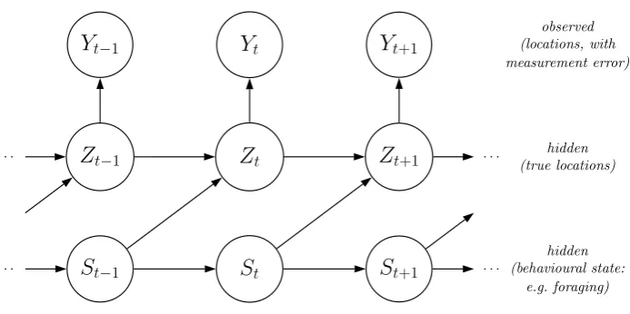
Let the state-dependent process be denoted by{Zt}Tt=1, with realizations zt = (lt, φt), where lt is
the step length in the interval [t, t+ 1] andφtis the turning angle between the directions of travel during
the intervals [t−1, t] and [t, t+ 1], respectively. Furthermore, let the underlying nonobservableN-state
Markov chain be denoted by{St}Tt=1. In the most basic model, the dependence structure is such that,
given the current state ofSt,Ztis conditionally independent from previous and future observations and
states, and the (homogeneous) Markov chain is of first order (Figure 1). We summarize the probabilities
of transitions between the different states in theN×N transition probability matrix (t.p.m.) Γ= (γij),
whereγij = Pr St=j|St−1=i
row vectorδ, where δi = Pr(S1=i),i= 1, . . . , N.
[Figure 1 about here.]
HMMs for animal movement data typically involve the additional assumption of contemporaneous
conditional independence (Zucchini et al., 2016). That is, conditional on the current state, the
step-length and turning-angle random variables are assumed to be independent:
fi(zt) =f(zt|St=i) =f (lt, φt)|St=i=f(lt|St=i)f(φt|St=i).
(Here and elsewhere we use f as a general symbol for a density function.) This assumption greatly
facilitates inference, yet is not overly restrictive. In particular, the two component series will still be
mutually dependent, because the states induce dependence between the component series. Plausible
distributions for modelling the circular-valued turning angles include the von Mises and wrapped Cauchy.
Step lengths are, by nature, positive and continuous, which renders gamma and Weibull distributions
plausible candidates for modelling this component.
Most of the HMMs considered in movement ecology thus far involve a two-state Markov chain, where
each state is associated with a different correlated random walk (CRW) pattern. CRWs involve
correla-tion in direccorrela-tionality and can be expressed by a turning-angle distribucorrela-tion with mass centred either on
zero (for positive correlation) or onπ (for negative correlation). The two states of the corresponding
models are often associated with the animal being either ‘encamped’ (with mostly short step lengths
and many turnings) or ‘exploring’ (with, on average, longer step lengths and more directed movement,
as expressed by smaller turning angles). This kind of labelling of the states should be made with
cau-tion; it is generally accepted that these states merely provide convenient proxies of an animal’s actual
behavioural state (see Section 7.4).
In movement ecology, it is usually of primary interest to relate the state-switching process to
envi-ronmental covariates, thereby investigating how individuals interact with their environment. This can
be achieved by considering a non-homogeneous Markov chain, with time-varying t.p.m.Γ(t) =γij(t),
linking the transition probabilities to the covariate vectors,v·1, . . . ,v·T, via the multinomial logit link:
γij(t)= Pr St=j|St−1=i
= PNexp(ηij)
k=1exp(ηik)
, (1)
whereηij =β
(ij)
0 +
Pp
l=1β (ij)
4.2
Inference for HMMs
For a homogeneous HMM, with parameter vectorθ, the likelihood is given by
LHMM(θ) =f(z
1, . . . ,zT)
=
N
X
s1=1
. . . N
X
sT=1
f(z1, . . . ,zT|s1, . . . , sT)f(s1, . . . , sT)
=
N
X
s1=1
. . . N
X
sT=1
δs1
T
Y
t=1
f(lt|st)f(φt|st) T
Y
t=2
γst−1,st, (2)
where we exploited the dependence structure in the last step. In this form, the likelihood involvesNT
summands, rendering its evaluation infeasible even for a small number of states,N, and a moderate
number of observations,T. This has led some users to believe that a Bayesian approach is required to
fit an HMM to movement data, often leading to the use of WinBUGS. This approach, in which the data
are augmented with the states at each time point, is computationally inefficient because the Markov
chains display high auto-correlation (see Section 5.6). Consequently, fitting HMMs to large movement
data sets is often infeasible when using Markov chain Monte Carlo (MCMC) in this way.
Returning to the likelihood of an HMM, it turns out that the use of a recursive scheme called the
forward algorithm leads to a much more efficient calculation than via brute force summation over all
possible state sequences as in (2). To see this, we define the forward probability of statej at time tas
αt(j) =f(z1, ...,zt, st=j), and the vector of forward probabilities at timetasαt= αt(1), . . . , αt(N).
The key point now is thatαtcan be calculated based onαt−1. More specifically, using the conditional
independence assumptions it can easily be shown that
αt(j) = N
X
i=1
αt−1(i)γijfj(zt).
In matrix notation, this becomesαt=αt−1ΓQ(zt), whereQ(zt) = diag f1(zt), . . . , fN(zt)
. Together
with the initial calculation α1 = δQ(z1), this is the forward algorithm. Rather than separately
con-sidering all possible hidden state sequences, as in (2), the forward algorithm exploits the dependence
structure to perform the likelihood calculation recursively, traversing along the time series and updating
the likelihood and state probabilities at every step. Such efficient recursive computation is one of the key
reasons for the popularity and widespread use of HMMs – the same trick can be applied to forecasting,
state decoding (see later) and model checking. The main price to pay for being able to rapidly conduct
such analyses is that the Markov assumption needs to be made for the state process. This assumption is
somewhat unrealistic in many applications, but is a good example of attempting to identify the correct
balance between complex models that try to mimic as many aspects of the data as possible, often at the
expense of becoming computationally intractable, and overly simplistic models such as the L´evy walk
The forward algorithm can be applied in order to first calculateα1, then α2, etc., until one arrives
atαT, the sum of all elements of which obviously yields the likelihood. Thus,
LHMM
(θ) =αT1t=αT−1ΓQ(zT)1t=. . .=δQ(z1)ΓQ(z2). . .ΓQ(zT)1t, (3)
where1∈RN is a row vector of ones. The computational cost of evaluating (3) islinearin the number
of observations,T, such that a numerical maximization of the likelihood becomes feasible in most cases.
Technical issues arising in the numerical maximization, such as parameter constraints and numerical
underflow, are straightforward to deal with (Zucchini et al., 2016).
A popular likelihood-based alternative is given by the expectation-maximization (EM) algorithm.
The EM algorithm also involves an iterative scheme for finding the maximum likelihood estimate, by
alternating between updating the conditional expectation of the states (given the data and the current
model parameters), and updating the model parameters based on the complete-data log-likelihood where
the unknown states are replaced by their conditional expectations. We do not elaborate on EM here,
since we agree with MacDonald (2014) in there being no apparent reasons to prefer it over direct
likelihood maximization, which is easier to implement.
From a Bayesian perspective, the efficient evaluation of the likelihood is also a great advantage.
There is then no need to augment the data with the unknown states: we can simply use the likelihood
as above, applying the forward algorithm, and carry out either a simple MCMC algorithm over the
parameter space, such as random walk Metropolis-Hastings, or direct numerical maximisation over the
(log) posterior density, if approximating the posterior distribution near its mode is adequate.
Of course, an analysis of movement data using HMMs does not end with estimating the model
parameters, and the HMM toolbox offers a variety of additional inferential techniques. In particular,
this includes the Viterbi algorithm, which is a recursive algorithm for “state decoding” — i.e. identifying
the most likely state sequence to have generated the observed time series, under the fitted model.
Furthermore, the forward and backward probabilities can be used to perform state prediction (i.e.
calculate the state probabilities at a given time) and to calculate “pseudo-residuals” (also known as
quantile residuals) for model checking. For more details, we refer to Zucchini et al. (2016).
4.3
Real data example: daily movement of elk
To illustrate the HMM approach to modelling animal movement, we re-analyze the elk data
dis-cussed in Morales et al. (2004). The data set was downloaded from the Ecological Archives (http:
//www.esapubs.org/archive/ecol/E085/072/elk_data.txt). We note that this new analysis is
nei-ther an attempt to replicate nor an attempt to improve the models discussed in detail by Morales et al.
(2004). The data set comprises four tracks, each with daily observations and several associated habitat
covariates. There are 735 observed locations in total. For more details, see Morales et al. (2004).
We fitted a joint two-state HMM, with von Mises turning angle and gamma step length distributions,
to all four elk’s tracking data, assuming all model parameters to be common to all individuals. About
2% of the step lengths were exactly equal to 0, which we accounted for following McKellar et al.
(2015) by including additional parameters specifying state-dependent point masses on 0 in the otherwise
strictly positive (gamma) step length distributions. To illustrate the type of ecological inference that
can be made using HMMs, we additionally implemented an AIC-based forward selection of covariates
influencing the state-switching dynamics, as in (1), which led to the inclusion of exactly one covariate,
namely “distance to water” (∆AIC compared to the baseline model without covariates: 11.3). This
latter type of inference, i.e. the fact that HMMs can easily be used to relate the evolution of an animal’s
behavioural states to environmental and habitat conditions, is what most often motivates the use of
HMMs for analyzing individual animal movement data (see, e.g. Morales et al., 2004, Patterson et al.,
2009, McKellar et al., 2015, DeRuiter et al., 2016).
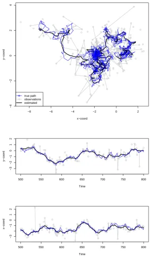
Figure 2 displays the estimated state-dependent step length and turning angle distributions, as well
as the estimated effect of the distance to water covariate on the t.p.m. The state-dependent mean step
lengths were estimated as 0.36 and 3.53 in states 1 and 2, respectively, and the associated estimated
turning angle distributions indicate a tendency to reverse direction in state 1 and directional persistence
in state 2. It seems reasonable to follow Morales et al. (2004) and label the two states “encamped”
and “exploratory”. The fitted model indicates that the probability of switching from “encamped” to
“exploratory” was highest when close to water, while the probability of a reverse switch was highest when
away from water (at the times the elks were located)—according to the fitted model, the “exploratory”
state is hardly ever visited when at distances to water greater than three kilometres.
[Figure 3 about here.]
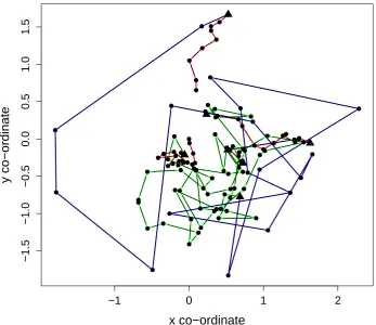
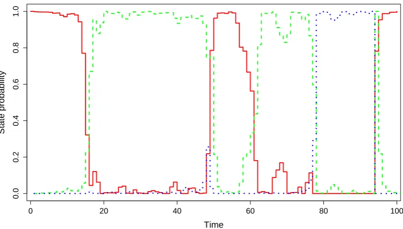
Figure 3 displays, for elk-287, the state sequence that is most likely to have generated this elk’s
observations, under the fitted model. This sequence was obtained using the Viterbi algorithm. Notably,
this elk was within 1 km of water for the first 89 days of observation (not shown in the figure)—during
which the animal frequently switched between the “encamped” and the “exploratory” state—and>1
km away from water on days 90-164—during which the animal only occupied the “encamped” state.
4.4
Limitations of the HMM framework
The HMM framework is well suited to deal with animal positions that a) are observed at regular temporal
spacings (and where the sampling unit needs to be meaningful with respect to the biological question of
interest) and b) are observed with only negligible observation, or in this specific case, positional, error.
Regarding a), it is straightforward to fit HMMs when data are missing at random on an otherwise
regular grid. However, if the sampling protocol varies, or if observations are made essentially at random
times, then the HMM machinery is not suitable. Discrete-time Markov chains are meaningless without
for example a step length distribution that takes into account the amount of time passed between
consecutive observations in a sensible way. (Note, however that there can be meaningful sampling units
that do not involve a regular temporal grid, e.g. positions observed each time a marine mammal comes to
the sea surface, such that the sampling is done on a dive-by-dive basis.) Continuous-time HMMs, with
the underlying Markov process operating in continuous time, do exist (see, e.g. Jackson and Sharples,
2002), but they are only suitable if the observed process has the “snapshot” property, such that thek-th
observation, made at timetk, depends only on the state active at timetk and not on the entire state
trajectory over the interval (tk−1, tk]. While this snapshot property is often naturally met in medical
studies, this is generally not the case for the kind of movement data typically analyzed.
Regarding b), when there is non-negligible measurement error in the locations—i.e. error that is
too large relative to the step lengths and/or the question of interest to be ignored—then the basic
HMM machinery is also not suitable. (If the locations are observed with error, then there is error in
the step lengths and turning angles, and the way this error is generated does not allow for the use of
say a simple convolution of step length and error distributions to be accommodated within the
state-dependent process.) In the next section, we will first discuss how a class of models that is closely related
to HMMs, namely state-space models (SSMs), can be utilized in order to deal with such positional error.
At the end of that section, we will also return to a), the problem of irregularly spaced observations.
5
State-space models: discrete time, measurement error
5.1
Model formulation
SSMs are doubly stochastic processes that are very closely related to HMMs. They have precisely the
same dependence structure, with an observed time series such that any observation depends only on
the current value of an underlying unobserved Markov state (or system) process. This can be generally
expressed as
zt=f(zt−1, εt), (4)
yt=g(zt, ηt), (5)
where the underlying latent state at time t is given byzt and the (typically noisy) observation of the
latent state isyt. The functionsf(·) andg(·) are the process and observations models, respectively, and
εandηare the process and observation errors, respectively.
Some authors regard HMMs and SSMs as the same (Capp´e et al., 2009). However, the label HMM is
usually used to indicate a model with a finite number of possible states, whereas in SSMs, the underlying
state process typically takes continuous values and hence involves an infinite number of states. In the
literature on movement modelling via state-switching processes, SSM approaches typically include both
using the link to the observations to describe potential measurement error (see Jonsen et al., 2005, or
Patterson et al., 2008). In contrast, in HMM approaches, as applied to GPS data, the measurement
error is often assumed to be negligible, so that the hidden component of the model involves only the
behavioural states, with the observed process giving the observed movement metrics, typically step
lengths and turning angles. While this may be acceptable for GPS data, which are generally very
precise, it will not be for other types of tag data such as that involving the use of satellite tags or
light-based geolocators.
We illustrate simple SSMs using Figures 4 and 5. Figure 4 shows an SSM that is a straightforward
extension of the HMM in Figure 1 to allow for measurement error in the step lengths and turning angles.
Herestis the (discrete) state at timet, as before, andztis the vector of (continuous) state-dependent
variables at timet, in this case the step length and turn angle. However, unlike in Figure 1,ztis not
observed directly, and so is modelled as a latent variable; togetherxt={st,zt}forms the hidden state at
timet. Here,ytis the observed step length and turn angle at timet, related to the true values through
the observation process. In practice, however, this model may not readily be applied: in particular
errors in turn angle and step length may be temporally correlated. Nevertheless, for tags that measure
speed (or acceleration) and bearing, rather than absolute location, models of this type, that include
a component for measurement error in these quantities, may be useful (see Laplanche et al., 2015).
Typically, it is more natural for SSMs to model the true location of the animal as one of the hidden
states, rather than the step length and angle; this provides a more direct link to the noisy observations
on animal location that are provided by some types of tag (e.g. satellite/GPS tags) and it also allows
for more explicit inferences about animal location. This formulation is shown in Figure 5: here zt is
true location andyt is observed location. Models that include elements of both formulations are, of
course, possible—for example given a marine mammal tag that measures speed, orientation, depth and
occasionally horizontal position (when the animal surfaces), one may envisage a 3D model like that
of Figure 5 whereyt relates horizontal position and depth to true positionzt, but with an additional
observation model to link measured speed and orientation to change in true position.
[Figure 4 about here.]
[Figure 5 about here.]
In general, SSMs are much less mathematically tractable than HMMs. The likelihood for HMMs,
given in Eqn. (2), can be readily evaluated and maximized in the form of Eqn. (3). By contrast, the
likelihood for the model in Figure 4 is of the form
LSSM1(θ) =f(y
1, . . . ,yT)
=
N
X
s1=1
Z
z1
. . . N
X
sT=1 Z
zT
f(y1, . . . ,yT|z1, . . . ,zT)f(z1, . . . ,zT|s1, . . . , sT)f(s1, . . . , sT)dzT. . . dz1
=
N
X
s1=1
Z
z1
. . . N
X
sT=1 Z
zT
δs1
T
Y
t=1
f(yt|zt)f(zt|st) T
Y
t=2
and for the model in Figure 5 is similarly
LSSM2(θ) =
N
X
s1=1
Z
z1
. . . N
X
sT=1 Z
zT
f(z1)δs1
T
Y
t=1
f(yt|zt) T
Y
t=2
f(zt|zt−1, st−1)γst−1,stdzT. . . dz1. (7)
It is clear that evaluation of Eqns. (6) or (7) requires difficult (multi-dimensional) integrations;
closed-form expressions are only available in special cases, where the integrands are of a particular closed-form, such as
the linear normal models of the Kalman filter, described below. In other cases, model fitting is achieved
using computer simulation-based methods within the Bayesian inference paradigm. Two important
exceptions are (1) the use of Laplace approximations to approximate the required integrals within a
mixed-effects framework, and (2) discretization of the continuous states so that HMM machinery can be
used. In the next sections we describe briefly each of these approaches, starting with the Kalman filter,
then discussing the mixed effects and discretization approximations, before considering two Bayesian
inference methods: particle filters and Markov chain Monte Carlo.
5.2
Kalman filters
The Kalman filter (Kalman, 1960) is applicable in the special case of an SSM where the posterior
distri-bution of the state, conditional on the previous observations, is analytically tractable. This tractability
stems from two crucial assumptions: (1) that both the process and observation models are linear, and
(2) that their respective error processes are Gaussian. The Kalman filter also is a recursive (and
inher-ently Bayesian; see Wikle and Berliner, 2007) algorithm, updating state estimates while step-by-step
traversing along the time series. Again analogous to the forward-backward algorithm in case of HMMs,
the so-called Kalman smoother can be used to obtain state estimates given all observations and a fitted
model. A good exposition of the Kalman filter is given by Harvey (1990). Its development was a huge
breakthrough in the application of state-space models to problems in engineering such as radar tracking,
and has been applied to a vast number of problems in many fields. The Kalman filter and associated
variants thereof have also been applied to animal movement data. In particular, one of the most widely
used Kalman filters has been developed by Sibert, Nielsen and colleagues in a series of papers
(Sib-ert et al., 2003; Nielsen et al., 2006; Nielsen and Sib(Sib-ert, 2007) which tackle the problem of estimating
the position of animals (chiefly marine species) using ambient light data. Patterson et al. (2010) and
Johnson et al. (2008b) used Kalman filtering to correct positional errors in satellite telemetry data from
Service Argos. Indeed, Service Argos now employ Kalman filtering routinely to infer a most likely path
from Doppler measurements from Platform Terminal Transmitter (PTT) devices (Lopez et al., 2014).
5.3
Random effects approaches to SSMs
The SSM formulation is a natural way to view the joint problem of estimation of latent states given
uncertain data—and it fits very naturally to animal movement problems. The major barrier to the
linear SSMs are relatively complex for “end users”, whose capacity to deploy SSMs may be limited by
complexity of the necessary statistical machinery used to fit them. A relatively new approach to fitting
SSMs offers analysts a more straightforward and flexible path to develop relatively flexible SSMs via
mixed effects modelling. In this section we closely follow the description given in Fournier et al. (2012).
The usefulness of this approach comes through the ability to cast the SSM as a more general
hi-erarchical random-effects (or mixed-effects) model. In this case the latent states are random effects,
Z={z1,z2, . . . ,zT}. A model for the dataYT ={y1,y2, . . . ,yT}, conditional on the unobserved
ran-dom effects, is given asfYT|Z(YT|Z, θy) along with a model of the unobserved random effectsfZ(Z|θz).
It is immediately obvious that these two components are equivalent to the usual SSM components of the
observation and process models. From this, the joint density of both the latent states (random effects)
and observations conditional on the parametersθis
fZ,YT(Z, YT|θ) =fZ(Z|θz)fYT|Z(yT|Z, θy). (8)
However, for estimating the parametersθ={θz, θy}we require the marginal likelihoodLM(.). Obtaining
this requires integrating over the unobserved random effects
LM(θ|YT) =fYT(YT|θ) =
Z
RT
fZ,YT(Z, YT|θ)dZ. (9)
In the software packages ADMB-RE (Fournier et al., 2012) and Template model builder (Albertsen
et al., 2015), the Laplace approximation is used to calculate a fast approximation of Equation (9),
carried out as follows:
LM(θ;y) =
Z
L(θ;z, y)dz
≈
Z exp
l(θ;z, y)−12(z−ˆzθ)T(−lzz00(θ;z, Y)|z=ˆzθ)(z−zˆθ)
dz
= L(θ;z, y) Z
exp
−12(z−zˆθ)T(−l00zz(θ;z, Y)|z=ˆzθ)(z−zˆθ)
dz
= L(θ;z, y)·(2π)n/2
·det (−lzz00(θ;z, Y)|z=ˆzθ))
−1
2,
by taking the logarithm
lM(θ;y) =l(θ;z, y)−
1
2log (det (l
00
zz(θ;z, Y)|z=ˆzθ))) +
n
2 log(2π). (10)
In ADMB-RE and TMB, automatic differentiation is used to compute the Hessian matrix,l00uu(θ;u, Y)|u=ˆuθ
of the likelihood function, and minimization is done using standard numerical methods. This avoids
numerical approximation of Hessians and gradients, which can lead to poor optimization performance
through propagation of errors in numerical differencing schemes.
fisheries science for fitting population dynamics models (Maunder et al., 2009), they are only starting to
be more widely used in general ecology and only very recently in movement ecology. A recent paper of
Albertsen et al. (2015) has applied these estimation methods to demonstrate estimation of a CRW model
which incorporates an Ornstein-Uhlenbeck process on the velocity component. The authors provide an
R package argosTrack which applies these methods to Service Argos satellite telemetry data. This
model is essentially an extension of the CRAWL package (Johnson et al., 2008a), which used Kalman
filtering/smoothing of speed filtered Service Argos data. However, by specifying the movement model
within a mixed effects model framework, the restriction of Gaussian error terms no longer applies, and
Albertsen et al. (2015) demonstrate a model witht-distributed errors. We feel the mixed effects approach
to fitting SSMs in movement ecology is an exciting and productive way forward as it offers a fast and
flexible method for estimating a range of movement models. Initially, and like the Albertsen et al. (2015)
paper, the primary application will be in constructing more flexible error correction filters. However, it is
likely that models with more ecologically interesting process dynamics could be constructed within this
modelling approach. This sort of hierarchical state-space modelling has previously only been available
via complicated and bespoke modifications to Kalman filters (see e.g. Meinhold and Singpurwalla,
1989) or with MCMC sofware (e.g. WinBUGS, OpenBUGS, JAGS). These are discussed in papers by
Jonsen et al. (2013) and Jonsen et al. (2006) (and see Pedersen et al., 2011b, for a general comparison
of techniques and software).
As an illustrative example, consider a simple 2-dimensional problem. Let zt = (z1,t, z2,t) be a
2-dimensional state variable (e.g. longitude and latitude, easting and northing, etc.).
zt = zt−1+ηt, ηt∼N(0,Σz),
yt = zt+εt, εt∼tν(0,Σy).
We simulate 2000 observations from a random walk with independent process errors Σz = Iσz2.
To demonstrate how the approach extends the canonical linear Gaussian case, we simulated a noisy
heavy-tailed (t-distributed with degrees of freedomν) observation process Σy =Iσ2y with 40% of times
having missing observations. Results are displayed in Figure 6. This could not be accommodated using
a standard Kalman filter. The packageTMBwas used to estimate the model parameters.
[Figure 6 about here.]
5.4
Discretising space in SSMs
In this approach, the continuous latent variables are finely discretized, so that the complexities of
integrating over hidden states are reduced to a summation. The standard HMM machinery can then
be applied as described in Section 4. This is a powerful and underutilized approach which also has the
advantages of being able to incorporate non-trivial spatial constraints such as animals having to avoid
land-avoidance in marine species). These methods were first demonstrated for geolocation from depth
and temperature sensing tags by Thygesen et al. (2009) and Pedersen et al. (2008) and typically involve
the use of data from sensors as well as (or instead of) noisy estimates of x-y position. The sensor
data may be compared to spatial fields and a data likelihood can be generated for all states in the
state space. From there the standard HMM routines can be applied. The case with Markov switching
between diffusive and ballistic travel modes was shown by Pedersen et al. (2011a). In all these studies, the
transitions between latent states is governed by a PDE which is solved numerically to predict movement.
A comparison of these methods to non-spatial / behaviour-only HMMs and switching CRWs fitted using
MCMC, is given in Jonsen et al. (2013). A limitation of spatial HMM approaches is that, given the
large number of states which may need to be stored, computational aspects can be important.
5.5
Particle filters
Particle filtering is a widely-used technique in computational statistics for making Bayesian inference
from nonlinear SSMs where the emphasis is on “online” (i.e. real-time or near real-time) estimation
of the underlying states—in our case, the true, but unknown, animal positions and behavioural states
(where the application would be real-time tracking or location forecasting). It is less commonly applied
to offline or parameter estimation problems, although it can be used for both. The nomenclature is not
standardized in this area, and particle filtering is also referred to as sequential importance sampling and
sequential Monte Carlo. Like Markov chain Monte Carlo (MCMC, described in section 5.6), particle
filters can be used to make inference from very complex multi-state movement models. Two strong
advantages of particle filtering are (1) that it is very easy to set up the algorithm, requiring simply that
one can simulate from the movement model and can evaluate the likelihood of observations given states,
and (2) particle filtering can be fast to run compared with MCMC. However, when parameter inference
is required, as is commonly the case in movement modelling, these advantages typically disappear. A
practical disadvantage for practitioners is that general particle filtering software is not typically available,
requiring custom-written code.
The starting point for both the particle filtering and MCMC approach to Bayesian inference on SSMs
is to augment the set of model parameters to include additional auxiliary variables corresponding to the
latent states–i.e. the true locations of individuals and their behavioural states—which we denotex=
{z,s}={z1, . . . ,zT, s1, . . . , sT}. Further, we specify an initial latent state,x0={z0, s0}, corresponding
to the location and behavioural state at time 0. Using Bayes theorem, the joint posterior distribution
of the augmented model parameters, given the observed positionsy can be written
π(θ,x|y) ∝ g(y|x, θ)f(x|θ,x0)p(θ,x0)
=
T
Y
t=1
The (marginal) posterior distribution of the model parameters is obtained by integrating out the
aux-iliary variables. The necessary integration is, however, analytically intractable.
Particle filtering (and MCMC) both work by generating samples from the posterior distribution
π(θ,x|y). Inferences about model parameters, including latent states, is then made readily using tech-niques of Monte Carlo integration—for example, the posterior mean ofθ,zorscan be estimated from
the mean of the sample values. Both methods are described in many texts, but a good general
intro-duction is Liu (2004). Introductory articles to particle filtering include Doucet et al. (2000), Doucet
et al. (2001), and Arulampalam et al. (2002), and a very basic application to a state-switching animal
movement model is given by Patterson et al. (2008).
Particle filtering generates independent samples from the posterior. There are many variants, but
the most basic, the bootstrap filter, can be viewed as an extension of importance sampling. There, many
replicate samples are simulated from a proposal distributionq(), and each is assigned an importance
weightw=π(θ,x|y)/q(); the weighted samples can then be used to make inferences about the posterior
distribution of interest. These samples are called “particles” in particle filtering. The bootstrap filter
makes three extensions:
1. Advantage is taken of the Markovian nature of the model, so that the algorithm proceeds one
time step at a time, starting by proposing values for time 1 based on an initial sample for time 0,
calculating time-specific weights,w1, and resampling (see next extension, below), then proposing
values for time 2 based on the samples at time 1, calculating weightsw2 and resampling, etc.
2. There is a resampling step at each time period, where the weighted particles are resampled with
replacement with probability proportional to the weight, to yield an unweighted set of particles
that can be used for inference.
3. The initial sample at time 0 comes from the prior p(θ,x0), and the proposal each time step is
based on the process model qt =f(xt|xt−1, θ). This results in a weight of a very simple form:
wt=g(yt|xt, θ), i.e. the observation process density.
The filtering algorithm outlined above is also accompanied by a reverse algorithm, the particle
smoother, that is exactly analogous to the backward step of the forward-backward algorithm in HMMs
and the Kalman smoother in Kalman filtering. This second stage is not relevant for online problems,
but is typically applied in offline problems like post-processing animal movement data.
Hence, all that is required to implement the most basic particle filter (and smoother) is the ability to
sample from the prior distributions of model parameters and latent states, to simulate realizations from
the process model, and to evaluate the observation process density given values of the latent variables.
Unfortunately, the basic method can suffer from high Monte Carlo error, because resampling with
replacement at each time step from the particles simulated at time 0 inevitably means that there are
fewer and fewer of the unique “ancestral” particle remaining at each time period—a phenomenon known
time-varying) components of the process model, such as animal locationszt and behavioural statesst,
because simulating stochastically from the proposal distribution (i.e. the process model) at each time
step generates new diversity among the simulated particles. However, for the static model parameters,
θ, each time resampling is performed, fewer and fewer unique values from the original simulated set
remain, resulting in an increasingly poor approximation to the posterior distribution. One solution to
this is to make the model parameters time varying, for example by having expected speed and turn angle
evolve slowly over time according to a first order Markovian process. This is the solution adopted by
some authors, e.g. Dowd and Joy (2011). Another solution is to extend the particle filtering algorithm
to maintain diversity among particles in static parameter values, for example by resampling from kernel
smoothed estimates of the joint posterior distribution of parameters or by introducing an MCMC step.
An example of an MCMC step, applied after particle filtering in order to facilitate static parameter
estimation, is Andersen et al. (2007). Many other techniques are available (see review by Kantas et al.,
2015); however, these methods tend to loose the advantages of simplicity and speed. Perhaps because of
this, or perhaps because of the absence of general software for particle filtering animal movement data,
MCMC (as described in the next section) has been historically the more popular approach.
5.6
Markov chain Monte Carlo
Markov chain Monte Carlo (MCMC) is a very popular approach for obtaining inference on the model
parameters within a Bayesian analysis by simulating (dependent) samples from the posterior distribution
(Eqn. (11)). Standard easy-to-use computer packages exist which implement an MCMC algorithm for
a given model, prior specification and associated data. The MCMC algorithm is performed within a
closed “black-box”, so that in-depth computational details of the algorithm are not required. The most
widely used packages for movement models are BUGS and JAGS (Lunn et al., 2000; Plummer, 2003).
Jonsen et al. (2005) provide BUGS code for fitting SSMs with multiple CRWs to animal movement data,
which has been employed widely. However, we discuss below why such general software packages can
perform poorly. Alternatively, bespoke MCMC computer codes can be written with complete control
over the updating algorithm, permitting more general updating algorithms (McClintock et al., 2012).
Typically this is a non-trivial endeavour.
The general structure of the MCMC algorithm for sampling from the joint posterior distribution
specified in Eqn. (11) is as follows. At each iteration of the MCMC algorithm, the model parameters,
θ, and auxiliary variables,x, are updated. For animal movement models, a mixture of single and block
updates are generally used. Single updates are typically used for the model parameters,θ, and discrete
behavioural state, st, at time t; and block updates for the true location of an individual at a given
timet,zt(i.e. the cartesian co-ordinates are updated simultaneously). Within the constructed Markov
chain, each iteration involves cycling through each individual model parameter, behavioural state and
location parameter (at timet) to update their values.
trial and associated probability for statei= 1, . . . , N,
pi =
f(zt, st=i|zt−1, st−1)f(zt+1, st+1|zt, st=i)
PN
j=1f(zt, st=j|zt−1, st−1)f(zt+1, st+1|zt, st=j)
(fort 6= 0, T). Thus a Gibbs sampler can be implemented, such that at each iteration of the Markov
chain the behavioural state is updated by simulating from the given Multinomial posterior conditional
distribution. For the remaining parameters, the full posterior conditional distribution is of non-standard
form so that a Metropolis-Hastings algorithm is used. For example, suppose that a given iteration of
the Markov chain, the current location at time t is zt (for t 6= 0, T). Simulate the proposed value,
v ∼ q(v|zt), where q is the proposal distribution. For example, a common choice for the proposal distribution is a random walk, such thatv =zt+, where E() = 0. The proposed value is accepted
with probability, min(1, A), where
A = f(zt+1|v, st, θ)f(v|zt−1, θ)q(zt|v)
f(zt+1|zt, θ)f(zt|zt−1, θ)q(v|zt)
,
using the Markovian structure of SSMs. If the proposed value is rejected the chain remains in the
same location state. The analogous Metropolis-Hastings updates are used for the remaining model
parameters. See McClintock et al. (2012) for further discussion of such updating algorithms, including
where transitions between states may be dependent on additional factors/covariates.
This form of updating leads to very high auto-correlation in the Markov chain for the simulated true
location states,zt. This is a direct result of the high correlation between the location of an individual
at time t, with their corresponding locations at time t−1 and t+ 1 (animals do not teleport). This can be immediately seen in the above acceptance probability for the Metropolis-Hastings algorithm
for updating the location of an individual at timet—the acceptance probability is a function of the
underlying density function for the movement of the individual in the intervals [t−1, t] and [t, t+ 1].
This leads to generally very poor mixing within the Markov chain, and low effective sample sizes, so
that large numbers of iterations are needed to obtain converged posterior estimates with small Monte
Carlo error. Consequently, extensive posterior checking should be conducted to assess the convergence
of the Markov chain, for example, using multiple Markov chains with over-dispersed initial values for
the model parameters and auxiliary variables. For further discussion of these issues for general SSMs
see, e.g. Fearnhead (2011).
Approaches have been proposed to improve the mixing of MCMC algorithms for SSMs. The most
notable (and promising) approach considers a particle MCMC algorithm that combines particle filtering
with MCMC (Andrieu et al., 2010). The model parameters,θ, and discrete states,sare updated using
an MCMC-type algorithm (for example a single-update Metropolis-Hastings within Gibbs algorithm)
and the true locations, z, updated using a particle filter. In addition, the behavioural states do not
necessarily need to be imputed within the MCMC algorithm. Assuming first-order Markovian transitions
joint density (i.e. likelihood) of the true locations, given the model parameters (see Eqn. (3)). In other
words the behavioural states do not need to be treated as auxiliary variables and imputed within the
MCMC algorithm.
Finally, we note that SSMs generally assume observations are recorded at a set of equally-spaced
discrete-time intervals. In practice, irregularly spaced time steps can be forced into the regular time
interval SSM framework by linearly interpolating the recorded location observations at the required time
steps (Jonsen et al., 2005; McClintock et al., 2012). Discrete-time models have the advantage of accessible
model-fitting tools (albeit potentially very inefficient) and immediately interpretable model parameters.
However, issues arise, for example, if there is a mismatch between times between observation and the
scale at which transitions occur between states. See McClintock et al. (2014) for an in-depth discussion
of the issues of discretising time. An alternative and more natural approach in many situations (though
at the expense of mathematical simplicity) is to consider continuous-time models, discussed in the next
section.
6
Diffusion models: continuous time
Continuous-time modelling of movement almost always makes use of diffusion processes—Markov
pro-cesses with continuous sample paths. We distinguish two broad approaches: one is to build models from
the limited selection of tractable diffusion models (Sections 6.1 to 6.4) and the other is to define models
directly in terms of the stochastic differential equations that they satisfy (Section 6.5). Our emphasis
here is on the former, with animals switching between different movement modes—the direct equivalent
in continuous time of the HMMs of Section 4.
6.1
Brownian motion
Brownian motion, or the Wiener process, the continuous-time version of a random walk model, is the
simplest diffusion process, and its density function can be written down explicitly. If a Brownian motion
W(·) starts at location0at time 0, then
W(t)∼N(0, tΣ),
where Σ is a variance-covariance matrix (or, for one-dimensional movement, just a variance), most
commonly with Σ = σ2I
d (the isotropic or circular case, with Id the identity matrix of order d).
Brownian motion is an extremely simplistic model, representing an animal having no interaction with
environment, and no directed or persistent movement. The model is of limited use in its own right, but
becomes a useful component in switching models (Section 6.4).
normal density;
L(Σ|{x(tj)}) =
Y
j
(2π)d/2|∆tjΣ|−1/2exp(−(∆x0j(δtjΣ)−1∆xj)/2),
where ∆xj =x(tj+1)−x(tj), ∆tj =tj+1−tj.
Brownian motion is often used as a purely local model. Horne et al. (2007) suggest that movement
between known locations can be estimated through the use of Brownian bridges; this possibility is
also implicit in Blackwell (1997, 2003). The Brownian bridge (B(t), t1 ≤ t ≤ t2) is the stochastic
process that arises from Brownian motion (W(t), t≥ 0) in which the state of the process is not only
known at the start of the process, but also at the end (Anderson and Stephens, 1996). The Brownian
bridge therefore describes Brownian motion conditioned on its state at these endpointst1andt2. With
endpointsB(t1) =aandB(t2) =b, the process has
B(t)∼N
a+ t−t1
t2−t1
(b−a),σ
2(t
2−t)(t−t1)
t2−t1
, (12)
fort1≤t≤t2(Anderson and Stephens, 1996). Specifically, this kind of interpolation can be informative
about an animal’s utilization distribution—the marginal distribution of its location—and hence about
its habitat use. Given two consecutive observations of location, it is assumed that the animal is moving
according to Brownian motion and so the only movement parameter is the random volatility. The theory
of Brownian bridges allows the likelihood of space use at any time between the two known locations to
be easily evaluated, given the volatility parameter of movement. Furthermore, given a series of locations
over time, disjoint Brownian bridges can be constructed between pairs of observations and the likelihood
can be evaluated due to conditional independence.
6.2
The Ornstein-Uhlenbeck position model
The Ornstein-Uhlenbeck (OU) process (U(t), t ≥0) is a stochastic process introduced by Uhlenbeck
and Ornstein (1930) as an improvement to methods for modelling the movement of particles—based on
Brownian motion (see e.g. Guttorp, 1995). This stationary, Gaussian process is mean-reverting (Dunn
and Gipson, 1977), and so has a tendency to drift towards its long-term mean. The equilibrium
distri-bution of a particle following an OU process inddimensions is
U(t)∼N(µ,Λ), (13)
where U(t) and µ are d-dimensional vectors and Λ is a d×d covariance matrix. The conditional
distribution of the process at a future point in time, given its current value, can be described as
whereU(t),µand Λ are as above and Bis a d×dstable matrix—that is,eBt
→0 ast→ ∞—so as to ensure a positive-definite covariance (Dunn and Gipson, 1977). It can therefore be seen thatµdescribes
the centre of the process, with rate of attraction towards the centre controlled byB and with random
variation governed by Λ.
The OU process is perhaps the simplest continuous-time model that is of use in its own right. It arises
from ecologists’ interest in learning about the home-range of an animal, the spatial range in which it
performs its daily survival activities (B¨orger et al., 2008)—often mathematically defined as the smallest
geographical area in which the animal spends a fixed proportion of time (Jennrich and Turner, 1969).
Approaches to estimating the home range include that in Jennrich and Turner (1969), proposing that an
animal’s utilisation distribution (see Section 6.1) can be represented as a bivariate Normal distribution.
This led to the first method for modelling animal positions in continuous time—given by Dunn and
Gipson (1977), who model the (X, Y) co-ordinate positions of an animal by a 2-D OU process. The
long-term position of the animal is described by the equilibrium distribution of an OU process— see
(13). Movement therefore has a random element to it, but the animal is ultimately attracted to a centre,
and so has a well-defined home-range. Autocorrelation of successive observations is accounted for by
the conditional distribution of the OU process—see (14).
In the application of the OU process to animal movement, the matrix B is often taken to be
isotropic—uniform in all orientations—withB=bId forb <0 to ensure stability. More general classes
ofB may be used, but note that the class must be symmetric under rotation and reflection, otherwise
there would be some significance placed on the co-ordinate system chosen (Dunn and Gipson, 1977;
Blackwell, 1997). For example, the general diagonal case is not appropriate, for this reason.
Inference for the OU parameters governing movement in Dunn and Gipson (1977) is carried out by
maximum likelihood methods. A difficulty presented by this method is the choice of likelihood for the
initial observation. Dunn and Gipson (1977) explore two approaches. One is to ignore the information
provided by the initial observation, effectively conditioning on that observation; this is the approach used
most widely in movement analysis. The other is to use the tractability of the equilibrium distribution
for the animal’s position and add a likelihood term assuming that the initial observation comes from
that equilibrium distribution. They discuss the implications in terms of statistical information, and the
relationship with the actual sampling scheme for the data.
The OU process addresses the problem of autocorrelation of position, meaning high frequency ‘bursts’
of observations can be modelled. The OU process however, will always result in an estimate of
home-range being elliptical and unimodal. For some animals and habitats this will clearly not be an
appro-priate assumption (Blackwell, 1997). Again, this limits the usefulness of the model on its own, but it is
6.3
The Ornstein-Uhlenbeck velocity model
The persistent movement modelled using correlated random walks (Section 4.1 can be extended to
a continuous-time framework. One such approach is given by Johnson et al. (2008a) and applied to
data from northern fur seals in Kuhn et al. (2009). Johnson et al. (2008a) model positions over time
indirectly, by formulating a model in terms of velocity—the instantaneous rate of change of location.
The behaviour of the velocity vector over time is then described by a bivariate OU process—in practice
Johnson et al. (2008a) use two independent 1-D OU processes. The persistence assumption on how
animals move is thus incorporated as a result of the autocorrelation of the OU process.
The location of the animal at any time,t, can then be found by integrating the velocity process up
to timet. This results in the location process no longer being Markovian—as in the OU position model
above—as it depends on the entire velocity process prior to timet. However, the combined process of
position and velocity is Markovian in this model. Observation error in position is incorporated into
Johnson et al. (2008a) via a SSM with Gaussian distributed errors and extended in Albertsen et al.
(2015) to allow for non-Gaussian errors.
Statistical inference for all unknown parameters in Johnson et al. (2008a) is carried out using
maxi-mum likelihood techniques. Kalman filtering—see Section 5.2—is used to find these maximaxi-mum likelihood
estimates, along with prediction intervals for the velocity and location of the animal at unobserved times.
In Albertsen et al. (2015) inference is carried out via the Laplace approximation using the R package
TMB.
6.4
Modelling switching behaviour in continuous time
Blackwell (1997) suggests an extension to the Brownian and OU models in order to allow for behavioural
‘switching’. As in the HMMs of Section 4, it is assumed that at any point in time an animal exhibits
one of a finite set of behavioural states. The process describing the behavioural state of the animal
is assumed to follow a continuous-time Markov process. The animal’s movement is modelled in the
same way as in Dunn and Gipson (1977) by an OU process. The OU process parameters however, are
dependent on the behaviour process; when the animal is in behavioural statei it moves according to
an OU process with the parametersµi, Λi, Bi (Blackwell, 1997)—see ( 14). Brownian motion can be
recovered as a limiting special case.
The Markov process M(t) taking values from a finite state-space of size N can be fully described
by its generator matrix,G={gij} fori, j = 1, . . . , N. The valuesgij, i6=j describe the infinitesimal
transition rate from state i to state j; the rate of transitions out of state i is given by −gii. The
process can therefore be thought of as being in a statei for a length of time exponentially distributed
with mean−1/gii, and then ‘switching’ to another state j with probability fori 6=j. An alternative
parametrisation (Guttorp, 1995) of the process is therefore given by the transition rates out of each
state,λ={λi}={−gii}, and the set of jump probabilitiesQ={qij}={ gij
−gii}fori6=j.