2D and 3D Geophysical Imaging of Polygonal Patterned Ground in the McMurdo Dry Valleys, Antarctica

Polygonal Patterned Ground in the

McMurdo Dry Valleys, Antarctica.

__________________________________

A project submitted in partial fulfilment of the requirements for the degree of

Master of Science in Geology at the

University of Canterbury by

Myfanwy Jane Godfrey

Department of Geological Sciences, University of Canterbury, Christchurch, New Zealand

The PPG found in the Dry Valleys is some of the oldest on the planet with ages of up to 8 million years assigned to them. The activity of some of these Antarctic PPG areas has come into question with the proposal that they may be the result of sublimation processes rather than actively re-working freeze and thaw processes.

Near surface geophysical methods of ground penetrating radar (GPR), resistivity tomography and electromagnetism have been applied to four Antarctic Dry Valleys polygonal patterned ground (PPG) areas; two in Victoria Valley and two in Beacon Valley. The aim was to resolve subsurface structure and activity of the PPG without disturbing the delicate permafrost soils.

Multiple techniques were used so that there could be greater reliability on the interpretations of this data without the need for damaging subsurface geological calibration of the geophysics by obtaining direct subsurface data through methods such as trenching or drilling.

Subsurface structure of the PPG was resolved; active layer depth, deformation of permafrost in the vicinity of contraction cracks and zones of attenuation were identified. Significant deformation in the subsurface horizons of the permafrost and associated with thermal contraction crack wedge growth was identified over PPG suggested to be formed only by sublimation in Beacon Valley, thus calling into question this interpretation of the PPG activity.

I must thank my other (field work) half Jon Lapwood – you were my rock (thanks Tracy and Connor for letting me borrow him). Thanks also to Michele Bannister who was a pivotal member of “team extreme”. Without both of these people it would have been impossible to surmount the difficulties posed during the 2006/07 K054 field season. The same sentiment must be said to Antarctica New Zealand for their remarkable professionalism and field support during my time in Antarctica. It was much appreciated at the time and still is now. In particular, Rob McPhail, the brilliant helicopter pilot who transported all our unwieldy geophysics gear between sites and provided me with some beautiful photographs of my field area.

I thank the Department of Geological Sciences at Canterbury University, my official supervisors David Nobes and James Shulmeister and my unofficial supervisor Ron Sletten. Thanks David Bell and Margaret Bradshaw for your input, and Steve Arcone for scaring the bejesus out of me and getting me in contact with James Doolittle (thanks as well). Thank you Jon Southward my computer guy, who is probably the most acknowledged man in the department. Masters students would despair without you.

Thank you to Greer Gilmer for your continual comic relief and never ending distraction from things I really didn’t want to do. The same goes for the rest of the geology crew graduating year 2006 you guys were the core of my university experience.

Thank you to the Mason Trust and the Federation of Graduate Women for financial support for my field work and conference attendance.

Thank you to my Grandparents, Ray and Shirley Milne for continuous cups of tea and home baking as well as a refuge when it was time for me to “throw my toys out of the cot”

Most importantly Thank you to my parents Megan and Robert Godfrey for allowing me the freedom to keep surprising you while secure in the knowledge that you love me enough to help me with whatever outcomes came from my decisions.

Thank you to all others who had a hand in helping me with this endeavour.

Frontispiece………. Abstract………... Acknowledgements... Table of Contents... List of Figures……….. List of tables……… 1: Introduction to this Thesis: background information and context for

this research……….. 1.1 Permafrost and Polygonal patterned ground:………. 1.1.1 Permafrost………... 1.1.2 Development of polygonal patterned ground………. 1.1.3 Target identification……… 1.2 Near surface geophysics in permafrost soils……….. 1.2.1 Physical properties of permafrost……… 1.2.2 Previous applications of near surface geophysics in Permafrost and in the Antarctic……… 2: Field area: The Dry Valleys………..

2.1 Introduction to the field area ………. 2.1.1 PPG in the McMurdo Dry Valleys……….. 2.1.2 Additional factors for use of near surface geophysics in the McMurdo Dry Valleys………...

2.4.1 VVP1………... 2.4.1 VVP2………... 2.4.3 BVP1………... 2.4.4 BVP2………... 3: Near surface geophysics……….... 3.1 Basic principles……….. 3.2 Ground Penetrating Radar………. 3.3 Resistivity………... 3.4 Electromagnetism………... 4: Methodology………. 4.1 General survey set up………. 4.1.1 Factors involved in working in the Dry Valleys…………. 4.2 Topographic Data………...

4.2.1 Data collection………. 4.2.2 Data processing………... 4.3 GPR……… 4.3.1 Data collection………. 4.3.2 Data processing………... 4.3.3 Data display……… 4.4 Resistivity………

4.4.1 Data collection………. 4.4.1.1 VVP1……… 4.4.1.2 VVP2……… 4.4.1.3 BVP1……… 4.4.1.4 BVP2……… 4.4.2 Data processing………... 4.5 Electromagnetism……….. 4.5.1 Data collection………. 4.5.2 Data processing………... 5: Results and interpretation……….

5.1.2 Resistivity tomography………….……….. 5.1.2.1 General comments……… 5.1.2.2 Subsurface features………... 5.1.3 Electromagnetism………..

5.1.3.1 General comments………..………. 5.1.3.2 Subsurface features………. 5.1.4 Synthesis………..………...

5.1.4.1 Active layer resolution………..….. 5.1.4.3 Contraction crack resolution….………. 5.1.3.4 Buried Massive Ice bodies and Relic surfaces…. 5.2 Resolution of seasonality in the subsurface (time-lapse)…………..

5.2.1 VVP2 time-lapse GPR……….... 5.2.1.1 General comments……… 5.2.1.2 Time-lapse trends…….……… 5.2.2 VVP1 time-lapse Resistivity tomography……….

5.2.2.1 General comments……… 5.2.2.2 Time-lapse trends……… 5.2.3 Synthesis………..………

Appendix IV: GPR data ………. Appendix V: Resistivity data ……….. Appendix VI: Electromagnetism data……….…….. ………..

Figure 2. Simple contraction crack development model (Lachenbruch 1963) Figure 3. Soil deformation movement between contraction cracks in polygonal

patterned ground

Figure 4. deformation within contraction crack Figure 5. target identification

Figure 6. Field area location: McMurdo Dry Valleys, Antarctica

Figure 7. topographic profiles of PPG cross sections of Victoria and Beacon Valleys showing differing ridge and crack heights from immature to mature PPG Figure 8. PPG in Victoria Valley

Figure 9. PPG in Beacon Valley

Figure 10. Victoria Valley survey area VVP1 characteristics

Figure 11. Victoria Valley survey area VVP2 topography and characteristics Figure 12. Beacon Valley survey area BVP1 topography and characteristics Figure 13. Beacon Valley survey area BVP2 topography and characteristics Figure 14. Ground penetrating radar technique summary

Figure 15. Diffraction curve generation in a step along GPR survey.

Figure 16. Common Mid point survey geometry and response relationships to velocity

Figure 17. Resistivity tomography “Wenner” array geometry

Figure 18. Generation of an electromagnetic response in the subsurface by using primary and secondary magnetic fields

Figure 19. The relationship between electromagnetic real and quadrature response. Figure 20. Topographic data collection

Figure 21. Alignment of GPR lines across the survey area Figure 22. Conducting GPR in the Dry Valleys

Figure 23. Common mid point semblance plot for velocity analysis Figure 24. Conducting Resistivity in the Dry Valleys

massive ice body in relation to the survey areas

Figure 32. Correlation of resistivity anomaly with GPR reflector in VVP2 Figure 33. time-lapse cubes showing increased resolution of strong subsurface

reflectors through the thaw

Figure 34. Summary of physical resolved physical properties of PPG subsurface and appropriate near surface geophysical techniques

Figure 35. Resistivity transect across Beacon Valley Figure 36. examples of Antarctic relate global systems Figure 37. Mars images of PPG.

List of Plates:

Plate 1. VVP1 GPR results Plate 2. VVP2 GPR results Plate 3. BVP1 GPR results Plate 4. BVP2 GPR results Plate 5. VVP1 Resistivity results Plate 6. VVP2 resistivity results Plate 7. BVP1 Resistivity results Plate 8. BVP2 resistivity results

Plate 9. VVP1 Electromagnetism results Plate 10. VVP2 Electromagnetism results Plate 11. BVP1 Electromagnetism results Plate 12. BVP2 Electromagnetism results

Plate 13. VVP2 GPR 100 MHz Synthetic aperture migration time-lapse results Plate 14. VVP2 GPR 200 MHz synthetic aperture migration time-lapse results Plate 15. VVP1 Resistivity time-lapse results South – North line 1

1: Introduction to this thesis; background information and

context of this research:

PPG is commonly a feature of permafrost environments. The two main forms of PPG are ice-wedge PPG and sand wedge PPG. Previous works on permafrost mechanisms have produced working models for the formation of polygonal patterned ground (PPG) (e.g. the iconic paper by Lachenbruch 1962) applicable in general to PPG. Whether ice wedge or sand wedge PPG is formed depends on the local area conditions such as water content, ground thermal regime, salt concentrations, and soil composition. In general ice wedge PPG is associated with humid permafrost conditions and is far more common (Black 1976). Most PPG areas in the Arctic are attributed to ice wedge processes. Sand wedge PPG is the product of arid permafrost conditions and Antarctica is classed as the coldest desert on Earth. Studies of PPG in the Arctic are only applicable in general terms to Antarctic examples.

The polygonal patterned ground (PPG) in Antarctica was first documented in 1904 by Robert Falcon Scott’s attempt on the South Pole (Scott 1905) but has not received as much scientific attention as its Arctic equivalent in the North. This is mostly due to the relatively short period of extensive research in the Antarctic as major scientific focus has only been since the International Geophysical Year (IGY) in 1957. There is also a lack of accessibility of the frozen continent as field work seasons are limited to southern hemisphere summer months November to February.

Antarctica is 98% covered in ice and any areas exposed are under strict environmental protocols under the Antarctic treaty. Research into PPG processes in ice free areas in Antarctica must limit the disturbance to the environment as much as possible. As such; to date, superficial trenching (<1.5m) and surface monitoring have been the most common research methods for examination of PPG subsurface structure and activity in the Antarctic. However they are highly invasive in this environment.

Specific PPG research targets associated with the chosen field areas are discussed, as well as the implications this research has for further geophysical PPG studies in the Antarctic.

Near surface geophysical techniques provide a means of interpreting changes in physical properties in the subsurface and relating them back to geological structures with no invasion and limited disturbance of delicate soils. Previous applications of near surface geophysical techniques (Arcone et al. 2000, Guigliem et al. Petterson and Nobes 2002, Davis 2002 etc) have shown that substantial subsurface data can be obtained by applying these techniques in the Antarctic environment. With the application of near surface geophysical techniques to Antarctic PPG in the McMurdo Dry Valleys it is expected that significant subsurface data on PPG structure and activity will be available.

Within the Dry Valleys two conflicting views dominate the interpretations of PPG surfaces: stable surfaces (e.g. Marchant et al. 2002) vs. active and re-working surfaces (e.g. Sletten et al. 2003). The survey areas in Victoria and Beacon Valley were chosen to expand on a theme of development progression of PPG processes. They represent the development of polygonal patterned ground from young and immature (Victoria Valley estimated age 104yrs) to old and mature PPG surface expression (Beacon Valley estimated age 106).

1.1 Permafrost and Polygonal Patterned ground:

In this section the basic terminology for understanding PPG is defined, and PPG processes are outlined. Factors such as the common physical properties of permafrost and PPG due to the formation processes are important for interpretation of the geophysical data collected for this research.

1.1.1 Permafrost:

The subsurface of permafrost soil areas can be divided into three main zones (Figure 1): the Active layer (sometimes referred to as a Talik(s) or freeze thaw zone),

Permafrost, and Permafrost base. These zones are based on horizons of temperature range and pore water phase. The definitions for terms relevant to permafrost and PPG are as follows:

Average annual ground temperature is required to be below zero for two consecutive years to be classed as permafrost.

Active layer occurs at the surface and represents the body of soil that has temperatures that vary from below 0ْ C during the freeze period to above 0ْ C during the thaw. The variation in soil temperature results in the freezing and thawing of pore water within this layer. This produces varied geophysical properties within the course of a season.

Permafrost is the zone below the active layer and above the permafrost base. Permafrost has soil temperatures permanently below zero. In permafrost pore water is permanently frozen and the material is often referred to as “ice-bonded”.

soil creates a soil temperature of 0ْ C. Therefore as climatic conditions get colder permafrost thickness increases and vice versa. This results in increased distribution and thickness of permafrost at cold climate, high latitudes, high altitudes, and in Periglacial environments.

Level of zero annual amplitude is where ground temperatures cease to vary over the seasons. This depth represents where climatic influences on the ground thermal regime cease to have effect.

1.1.2 The development of polygonal patterned ground

the research for this thesis was conducted, the PPG predominantly comprises sand wedge polygons. This is due to the arid nature of the Dry Valleys environment. Research on polygonal patterned ground received much attention in the 1960s and 1970s, predominantly by researchers such as Black and Berg (1963), Black (1976), Lachenbruch (1963) and Péwé (1974). The generalised mechanism for the formation of ice wedge and sand wedge PPG is similar but ice wedge formation has received far more attention in the literature. For example ice wedge PPG has been the focus of progressive studies by Mackay (1971, 1974, 1984, 1986, 1992, 1993, and 2000), whereas sand wedge PPG has no equivalent.

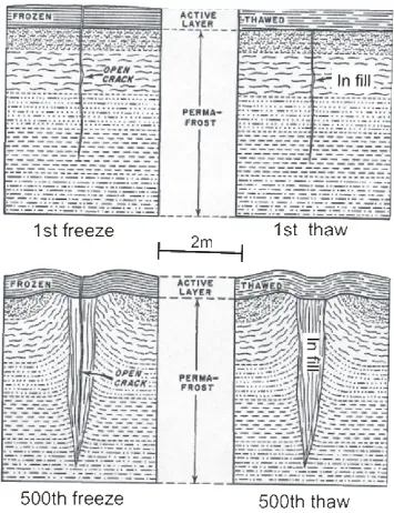
In general in PPG, thermal contraction and expansion of the soil volume over successive seasons forms a downward propagating crack. This contraction and expansion is within the top 5 – 10 m of permafrost and for contraction cracks to form the ground conditions must have a level of zero annual amplitude less than 5ْ C and seasonal temperature changes of 8-10ْ C (Black, 1976). Over a large area these cracks form a connected polygon (singular) or a network of polygonal patterned ground (plural). Figure 2 shows the theoretical development of an ice wedge in permafrost soils. When the ground is cooled horizontal tension in the soils is generated as soils attempt to contract. As soils are volumetrically constrained this tension in the soils is released as contraction cracks.

In extensive and continuous permafrost, contraction cracks develop into a network of interlocking polygonal structures, usually with six to eight sides and diameters of 1 – 25 m across (depending on local conditions and maturity of the PPG). Subsequent contraction re-opens the pre-existing cracks and forces propagation to depth to accommodate the thermal contraction. Mackay (1984) suggests that in early stage PPG development the re-opening of previous seasons’ cracks rather than generation of a new crack network the following season is the result of maximum stress being found at the bottom of the active layer. Therefore crack propagation is towards the

surface generated from the weakness of the previous season’s infilling material. The cracks expand further at the surface and accumulate more infilling ice and/or rock and soil material. With time and multiple seasons’ ice wedges develop. The development of this wedge geometry results in the deformation of the permafrost as the additional ice wedge volume is accommodated (Figure 3).

The deformation of the soils in the proximity of the thermal contraction crack wedge is displayed at the surface as raised edges. Figure 4 shows a model for the development of raised ridges within sand wedge PPG. This model is based on displacement of steel rods fixed into crack shoulders at 13 locations in the early 1960s by Robert Black (Sletten et al. 2003). In developed polygonal patterned ground the interlocking cracks and associated deformation ridges may show a “doughnut” surface geometry of raised edges and depressed centres.

1.1.3 Primary PPG structure target identification:

As outlined previously, the development of thermal contraction cracks and propagating infill wedges are the driving force behind the formation of PPG. Thermal contraction cracks are initially developed within the fluctuating active layer where temperatures vary above 0ْ C.

Figure 5 below summarises the primary targets of the PPG subsurface structure.

Time-lapse imaging will be targeting the changes in the subsurface through the warming/expansion period of the permafrost soils. This will specifically focus on changes in the active layer and thermal contraction cracks and associated ridges and their areas of influence.

1.2 Near surface geophysics in Permafrost soils.

The success of geophysical methods in permafrost soils will depend on the individual conditions of the area. The application of near surface geophysics to permafrost soils is varied, and has been concentrated primarily in Arctic environments.

1.2.1 Physical properties of permafrost:

Permafrost does not have a specifically measured set of geophysical responses as it is found in all soils and groundwater regimes provided that the climatic conditions remain cold enough to sustain permanent freezing of the soil. For the use of near surface geophysics the dominating physical properties of a body of permafrost will come from the general geophysical relationships such as: increased resistivity with grain size, degrees below 0ْ C and ice content (Haeberli, 1985). These factors are the standard relationships of geophysical response from the earth surface and will vary location to location according to the specific composition of the permafrost soils, source rocks, water content, and vegetation cover. Freezing may cause these properties to be varied from what might normally be expected. Salt and mineral concentrations within the soils may decrease the freezing point of the water content and skew the temperature – depth profile of the permafrost at specific locations. Frozen soils have different physical properties from their un-frozen equivalents primarily because water is constrained differently within the frozen structure. Freezing materials often results in an increase in resistivity/decrease in conductivity. Annan and Davis (1978) conducted laboratory tests with clay soils showing that as the temperature decreases there is a reduction of the dielectric constant (k).

velocities increase with decreasing temperature in materials containing water. This is due to the increase in density as the water content freezes, thus changing the physical properties with decreasing temperature. Further work on velocities by King (1984) refined this more to show that the increase in velocity was a function of “water-filled porosity” as it was discovered that significant amounts of water may remain unfrozen down to temperatures of -5 ْ C. Despite the low levels of ground water in Antarctic permafrost soils, this is important to note due to the poorly sorted gravely composition of the soils and high salt concentrations within pore water.

Although Arctic soil examples are useful for examining the potential for geophysics in Antarctica, there are issues surrounding the relative soil conditions found in these polar environments. Primarily the effect of free water within the soils is important when evaluating Antarctic examples. Antarctica is classified as a desert; the annual precipitation, in water equivalent measurements, across the continent is just 166 mm/year, and < 100 mm/year in the Dry Valleys (Doran et al. 2002). The lack of vegetation cover means that salt and mineral concentrations in the subsurface are higher as they are not used as nutrients for growth. Katabatic winds generated on the ice sheets maintain arid conditions by evaporating surface moisture and removing snow accumulations. These conditions create a barren, armoured rock strewn landscape with arid climatic conditions with little free water to be involved in permafrost processes. In general Antarctic permafrost soils have higher resistivities than their Arctic equivalents

1.2.2 Applications of geophysics in permafrost and the Antarctic:

(2008) present results from 3D GPR surveys of active and relic PPG structures in Alaska and mid west USA. Applications of geophysical techniques in the Antarctic soils has garnered results in the field of sedimentary and valley structure evaluations (e.g. Bristow et al. 2008, Arcone et al. 2003), and contaminant location (e.g. Pettersson and Nobes 2003). Near surface geophysics PPG studies have previously not been conducted in the Antarctic.

2: Field area : The Dry Valleys

This section focuses on the location of the field work that was conducted for this thesis. The environmental factors that may contribute to PPG formation and specific characteristics found at each field location are discussed. Working conditions and survey areas are described in the context of the geophysical results for PPG subsurface structure.

2.1 Introduction to the field area: The McMurdo Dry Valleys

Antarctica’s landmass is 98% covered in ice. The McMurdo Dry Valleys with an approximate area of 4800 square kilometres represents 95% percent of this 2% ice free area and the largest ice-free area of Antarctica. The McMurdo Dry Valleys is surrounded by the East Antarctic Ice Sheet (EAIS) to the West, North and South, which blocks and dams valleys, as found in Beacon Valley and Taylor Valley, and feeds into the Dry Valleys in the form of glaciers such as the Victoria and Taylor Glaciers. To the East, the McMurdo Dry Valleys are bounded by the McMurdo Ice Shelf which is part of the larger Ross Ice Shelf. McMurdo Dry Valleys are classified as a permafrost zone; subsurface soil temperatures are below zero degrees Celsius. The cold dry conditions found in the Antarctic are unique and although similar to frozen regions in the Arctic the lack of free water does result in variations within the permafrost. The Antarctic Dry Valleys have been suggested as the closest environmental analogue to the conditions found on Mars meaning that any research conducted there has implications for extraterrestrial applications.

Please note that although this thesis will refer to the American conventions of East and West Antarctica as seen in most Antarctic maps, maps will in fact be oriented for New Zealand as will any directional information such as East, West, North and South. For example the orientation of polygon surveys to the North, is North, consistent with longitude orientation and towards New Zealand.

2.1.2 Polygonal patterned ground in the McMurdo Dry Valleys, Antarctica.

The polygonal patterned ground (PPG) found within the McMurdo Dry Valleys is thought to be some of the oldest on the planet with estimated ages for some surfaces being of the order of 106 years (Sletten et al. 2003, Marchant et al. 2002). Black (1976) identifies the PPG in the Dry Valleys Antarctica as predominantly sand wedge and composite PPG. The established cold climate conditions and its polar position results in permafrost estimated to be between 240 – 970 m to permafrost base (Decker and Bucher 1980).

With the exception of the first identification of PPG in McMurdo Dry Valleys by Scott (1905), the literature surrounding PPG in Antarctica derives from the late 1950’s onward. Much attention was paid to Antarctic PPG in the 1970’s e.g. Péwé (1959), Black and Berg (1963, 1964, and 1966) Berg and Black (1966), Black (1973), and Ugolini et al. (1973). Recently literature has reflected an ongoing debate about the relative activity of PPG in the Dry Valleys. Sugden (1995) and Marchant (2002) propose that PPG surfaces in the Dry Valleys have been stable for millions of years, while Sletten et al. (2003) suggest that PPG surfaces in the Dry Valleys show evidence of growth and resurfacing.

patterned ground. Refer Figure 7 for a comparison of polygonal cross-sectional profiles from the two field locations and field site descriptions following.

Debate continues over the exact ages of the PPG surfaces in Victoria and Beacon Valley. Estimates for the ages of Victoria Valley are of the order of 104 years while Beacon Valley ages are on the timescale of 106 years.

Glacial history interpretations of the Dry Valleys use surfaces to produce ages for the advance and retreat of glacial movements through these areas. Interpretations of these surfaces are important for interpretations of glacial history.

Controversy over the age of PPG in the Dry Valleys is most evident in the interpretation of Beacon Valley PPG. Marchant et al. (2002) describes the PPG found there to be sublimation driven due to ice mass loss from an identified buried massive ice body (granite drift reference). Within the PPG of Beacon Valley is a subsurface tephra layer that has produced radiocarbon dates of circa 8 Ma. This tephra layer is recorded as being <1 m beneath the subsurface and relatively continuous across the areas studied in Beacon Valley (Marchant et al. 2002). If this tephra layer is in situ

PPG as actively reforming thus limiting the age of the surface at 1 – 2 million years. If the surface is actively re-forming then the tephra layer can not be considered to be a stratigraphic marker and any age associated with it cannot be used as a minimum age for the underlying buried massive ice body found within Beacon Valley. Hence the

activity of the PPG is central to the question of PPG age in Beacon Valley.

2.1.2 Additional factors for geophysical surveying of polygonal patterned ground in the Dry Valleys.

2.1.2.1 Delicate environment:

The McMurdo Dry Valleys are classed as an Antarctic Specially Managed Area (ASMA) with areas within the ASMA additionally identified as Antarctica Specially Protected Areas (ASPA). As such work conducted in the Dry Valleys undergoes strict environmental screening before permission to conduct the research is granted. All work conducted in the Dry Valleys must class their environmental impact as minimal and transitory. Classification of what is transitory impact is sometimes difficult in the Dry Valleys as environmental response times appear to be significantly longer than elsewhere in the world. This is most likely due to the lack of biological activity and cold short summer period reducing seasonality effects. Wind is a predominant re-working tool in the Dry Valleys but is only superficial in its effects. Significant subsurface disturbance such as trenching and drilling must have large scientific benefits to justify permission to be conducted in the Dry Valleys. As such the potential application of near surface geophysics to the identification of subsurface structures in the Dry Valleys is an issue which may provide a means of gathering additional subsurface information while limiting the disturbance of the environment. This thesis represents one possible ongoing application of these techniques in the Dry Valleys environment as a means of gathering subsurface data.

2.1.2.2 Mars Analogue:

identified on Martian surfaces at the Phoenix landing site using the High Resolution Imaging Science Experiment (HiRISE) program. Images from Mars show clearly formed polygonal patterned ground suggesting the presence of ice rich permafrost beneath the surface.

2.1.2.3 Climate Change:

Antarctica’s polar position makes it a hub for many global systems. For example, atmospheric circulation cells transfer heat and moisture from the equator to the poles ending in a permanent high pressure system over Antarctica, and the thermohaline conveyor belt global oceanic current is driven by the generation of Antarctic Bottom Water beneath the Antarctic sea ice and ice shelves. This combined with the relative lack of anthropogenic influences make monitoring changes in Antarctica a good way of monitoring human influences on Earth global systems. In Antarctica, the PPG is directly coupled with the atmosphere (Doran et al. 2002) due to the lack of overlying vegetation cover and isolation from anthropogenic influences on local conditions. Monitoring of PPG processes can thus be used as another tool for monitoring climate change.

2.1.2.4 Buried Massive Ice:

add a means of collecting additional information to glacial history interpretations and help with identifying future water sources on Mars.

2.2 Victoria Valley:

Victoria Valley is one of the three main valleys in the Dry Valleys and has the Victoria Glacier feeding into its Western extent (Figure 8 a.). The Victoria Valley is the northern-most of the Dry Valleys; valley floor elevations in our general field area ranged from 380m (ASL) near Lake Vida to 436m (ASL) at the foot of the Victoria Glacier.

2.2.1 Specific characteristics

The polygonal patterned ground found within Victoria Valley contained two distinct morphologies, one moderately developed with defined ridge and depressed centre geometries, and the other exhibited little to no ridge/crack relief. The moderately developed polygonal ground showed a larger range of clast sizes distributed at the surface with lateral sorting evident moving from coarser/larger clasts on the ridges to finer/smaller clasts within the depressed centre. The lateral sorting may be the result of freeze thaw frost heave processes or may simply be the result of katabatic wind sorting. The PPG surface did exhibit armouring where coarse clasts are concentrated at the surface as fine particles are removed by wind action thus protecting the underlying finer material. Polished sides to surface clasts that extended above the surrounding material were observed indicating the “sand-blasting” effect often associated with the formation of ventifacts in high wind environments such as the Dry Valleys during katabatic events.

2.2.2Field work location and environmental factors.

temperatures during our field season ranging from -11 to +6 degrees Celsius (field observations November/December 2006) Working conditions were mostly good with delays due to weather only occurring on one day due to low visibility (refer appendix 1 logistics report and activity log K054).

Figure 8: Views of Victoria Valley field locations a. above shows a ground photograph looking west towards Victoria Glacier which flows down from the East Antarctic Ice Sheet. Note the low topography of the PPG with Snow settling in the PPG depressions b., below shows an aerial view of the field site with X and Y marking the locations of VVP1 and VVP2 respectively. The PPG seen from this aerial view are approximately 8 – 15m from centre to centre.

a.

2. 3 Beacon Valley:

Beacon Valley is located at the southern end and in the inland reaches of the McMurdo Dry Valleys (Figure 5). Beacon Valley has the Mullins and Friedman debris covered glaciers feeding into the southern end of the valley while the northern end of the valley is dammed by the junction of the Turnabout and Taylor Glaciers.

2.3.1 Specific characteristics:

The Granite Drift and associated buried massive ice body found at the field site are suggested to be the result of a collision between those glaciers during the last glacial maximum when they extended down and into the main body of Beacon Valley (ref). The altitude of Beacon Valley is much higher than Victoria Valley with Beacon Valley floor occurring at an elevation of 930 m at the northern end and up to 1400 m at the southern end of the valley. The valley sides and surrounding mountain topography extends on average another 1000 m above the valley floor and reaches spot heights of > 2500 m (near Friedman Valley at the south end of Beacon Valley). From the valley floor the edges of the East Antarctic Ice sheet can be seen topping the valley sides. The proximity of the EAIS affected the weather conditions found within Beacon Valley with significantly stronger winds directed along the valley from the EAIS. The PPG observed in Beacon Valley exhibited high relief with well defined ridge/crack and depressed centre geometries.

2.3.2 Field work location and environmental factors.

surveying was not possible in Beacon Valley due to the loss of a team member to injury, but the unpredictable lengths of time required to complete one methodology survey in Beacon Valley would have made a systematic time-lapse survey difficult regardless.

2.4 Polygonal ground survey areas: identification and specifics

In total four areas of PPG were surveyed over the course of our 8 week field season. K054 also conducted cross-valley transects in conjunction with this PPG work, which will be referred to in the discussion of the results. The four areas of PPG range from “young” and immature PPG in Victoria Valley to “old” and developed PPG in Beacon. Two PPG areas were surveyed at each valley location: VVP1 and VVP2 represent the Victoria Valley PPG areas while BVP1 and BVP2 represent the Beacon Valley PPG areas. The specifics of the PPG survey areas and reasoning behind their selection is outlined in the following sections.

2.4.1 VVP1:

2.4.2 VVP2:

VVP2 was located in the moderately developed PPG on the floor of Victoria Valley. It exhibited moderately defined ridge and crack morphologies with relief within the survey area being between 0.5 – 0.75 m. The surface expression of the cracks were approximately 0.2 m across and showed a concentration of large clasts (generally elongate 0.1 - 0.2 m long axis length) infilling the crack. The associated ridges were well developed and encircled the corresponding depressed centre of the PPG area. The area was 20 x 12 m with the perimeter extending between these co-ordinates: NE corner E 161º 37.281 S º 77 20.159, NW corner E 161 º 37.253 S º 77 20.157, SE corner E 161 º 37.272 S º 77 20.169, SW corner E 161 º 37.243 S º 77 20.166 Figure 11 below shows the topographic data collected for correcting the geophysical data displayed in surface form to illustrate the morphology and geometry of VVP2.

2.4.3 BVP1:

The co-ordinates of the survey area are: NE corner E 160º 36.435 S 77º 50.999, NW corner E 160º 36.399 S 77º 50.994, SE corner E 160º 36.420 S 77º 51.004, SW corner E 160º 36.385 S 77º 51.000. BVP1 was of moderate to high surface relief and of a slightly irregular geometry with ridges not consistent with the classic polygon described in theoretical developments of PPG (Figure12). The survey area was 18 x 12 m and was located on the rim of a large depression approximately 75 m diameter. This depression may represent sublimation of the underlying buried massive ice body. The ground surface material exhibited intense iron staining creating a red brown landscape. The staining on the rocks seen at the surface made identification of the lithological composition difficult. Granites, granodiorites and beacon sandstones were identified in the survey areas. The ground material exhibited a range of clast sizes from fine sands to large boulders with larger clast sizes being concentrated at the surface. As seen in VVP2 there was sorting of the clast sizes across the polygon structure with smaller clasts being found within the depressed centre of the polygonal structure (Figure 12 b. – e.)

2.4.4 BVP2

3:

Near Surface Geophysics

This chapter will cover the basics of near surface geophysical techniques, theory and practise, so that the results and discussion presented here can be considered in context. Appropriate targets and the sensitivity of each method are discussed from a theoretical standpoint in the geophysical principles subsection. For a practical evaluation of the methods used in this research please refer to the methodology chapter.

3.1 Basic Geophysical principles:

Near surface geophysics is the use of techniques that measure the changes in subsurface physical properties within the Earth’s upper surface (100 m or so depending on the specifics of the method). Measuring these properties may involve putting a current into the Earth’s surface to measure electrical response, or may involve the propagation of a wave through the material, or may be related to creating a secondary magnetic field. The response from the subsurface is measured and recorded and is related to the physical properties of the underlying material.

The important physical properties that need to be understood for the use of near surface geophysics are:

Electrical conductivity: (σ) in siemens/meter (S/m) (inversely related to electrical resistivity (ρ) in ohm-meters (Ω/m)) is a measure of the ability of an electrical current to pass through a given volume of material. Electrical conductivity can be related to clay or water content within a subsurface lithology. Resistivity and electromagnetic methodologies are most relevant to this property but this is also linked to dielectric permittivity and so can effect electromagnetic wave propagation.

Magnetic susceptibility: (k) dimensionless and relates to the ability of a material to amplify an external magnetic field. The magnetic susceptibility is directly related to the concentrations of magnetic minerals, such as iron, within the subsurface. Most relevant to magnetic methodologies. The magnetic permittivity (µ) can effect the velocity of electromagnetic waves.

Density: (ρ) the mass of a material in a given volume, measured in kilograms/cubic meter (kg/m3). Density will effect the propagation of waves through a medium and changes in density will result in reflection and refraction of wave energies. εr is related to ρ and so this property can effect GPR propagation.

Different physical properties determine how energy will behave when interacting with subsurface materials. Each soil, lithology and rock type will have different physical properties depending on their individual geological parameters. Knowledge of how these physical properties relate back to geological parameters such as mineral compositions and water content can be used to image geological structures to great depth without physical invasion of the subsurface.

The loss of energy that occurs with depth is referred to as attenuation and it reduces the measurable responses that enable us to interpret subsurface conditions. Attenuation relationships refer to an attenuation constant (α) defined by:

α = ω {µaεa [(1 + σ2/ω2εa2 )1/2 – 1]/2}1/2

Where ω = angular frequency of the signal µa and εa = the absolute values of magnetic and electrical permittivity respectively and σ = conductivity (Milsom 2000)

It is important to note that when using geophysical methods that the data recorded relates to the physical properties and changes within these physical properties and may not directly correlate to changes within geological units. Ideally a drill hole or trench would be used to correlate physical response to geological units, but multiple techniques can also allow for greater control on geological interpretations.

Geophysical methodology has developed a number of ways to measure specific physical properties. The methods used in this research were ground penetrating radar (GPR), electrical resistivity tomography, and electromagnetic surveying.

3.2 Ground Penetrating Radar:

Ground penetrating RADAR (radio wave detection and ranging) is a wave propagation geophysical method used to resolve physical property changes within the subsurface by measuring two-way travel time of the reflected radar energy.

The energy used in GPR is electromagnetic containing a co-joined oscillating electrical and magnetic field which have the following relationship:

V = f λ

velocity of the wave through the ground is directly linked to the relative dielectric permittivity such that:

V = c .

√

(

µ

)

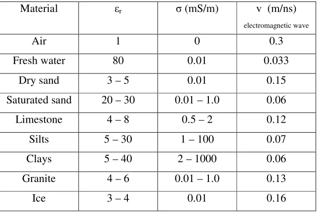
Since GPR waves are electromagnetic this relationship between electrical properties and velocity can affect the motion of the wave as it travels through the given material. This is commonly seen in increased attenuation of the signal through mediums with high conductivities. Table 1 shows the dielectric permittivity and conductivity in relation to the resulting electromagnetic wave velocity.

Table 1 Modified from Annan and Cosway 1992, and Milsom 2000, showing typical physical property values for some common materials relevant to applied geophysical methodologies.

GPR electromagnetic waves are commonly between 25 MHz to 1 or 2 GHz in frequency. The frequency values describe the central frequency (fc), as electromagnetic energy for GPR may be +/- 50% of the central frequency i.e. a 100 MHz signal will include electromagnetic energy down to 50 MHz and up to 150 MHz.

Electromagnetic waves are subject to reflection (where signal is “bounced” back

Material εr σ (mS/m) v (m/ns)

electromagnetic wave

Air 1 0 0.3

Fresh water 80 0.01 0.033

Dry sand 3 – 5 0.01 0.15

Saturated sand 20 – 30 0.01 – 1.0 0.06

Limestone 4 – 8 0.5 – 2 0.12

Silts 5 – 30 1 – 100 0.07

Clays 5 – 40 2 – 1000 0.06

Granite 4 – 6 0.01 – 1.0 0.13

subsurface) when travelling through a boundary where the physical properties of the two media are different (Halliday et al. 2002). It is reflection from buried boundaries that allows GPR to be used to create a subsurface profile of the physical properties which may be interpreted for geological information. Figure 14 shows how wave reflection and refraction as utilised in GPR.

Figure 14: GPR technique summarized: The transmitter (T) generates a pulse of electromagnetic energy that propagates to depth. Where boundaries between differing physical properties occur the energy is reflected to the surface and refracted to greater depth. Air wave, direct wave and reflected wave responses are detected by the receiver (R). The general survey parameters such as, stacking and time windows are controlled by a central unit which will also amplify and digitise the reflected signal to be saved and stored, or displayed. Modified Davis and Annan (1989), Reynolds (1997) Milsom (2000).

Reflection and refraction is generated at a boundary representing a change in properties. Signal reflected back towards the receiver is amplified digitised and stored (Davis and Annan 1989).

the reflected wave is rotated to a different orientation from the transmitted wave (Halliday et al. 2002).

Deeper reflections take more time to travel the wave path back to the receiver at the surface. The time taken to travel the reflected wave path is called the two-way-travel time. GPR traces plot the two-way-travel time and wave form of the reflected electromagnetic wave. The subsurface velocity can be used to convert two-way-travel time to accurate depth placements for a reflective boundary. Multiple GPR traces along a line can be used to create a profile cross-section of the subsurface.

The step increments at which the antennas are moved along a line must not exceed the nyquist sampling interval to avoid under-sampling and allow proper resolution of the subsurface feature targeted.

Nx = c / (4f √εr) = 75 / ( f √εr) (in m)

where c is the speed of light, f is the antenna centre frequency in MHz and εr is the relative permittivity of the host material.

As multiple traces from different step positions are collected, linear or planar reflectors within the subsurface display as lines, and point source reflectors plot as diffraction curves (Figure 15). The true dip of angled reflectors may need to be corrected for and diffraction curves may be collapsed to represent the original source geometry by using migration and a known velocity for the subsurface.

Figure 16: CMP step out geometry for collection of subsurface velocity data in the field. a) Antennas are stepped away from each other at a constant rate so that the increased distance the wave has to travel to reflect off appoint source is increased systematically b. shows an idealised resulting reflection profile where the relationship between antenna separation (and path length) is plotted against travel time between the antennas. CMP profiles show the arrival of the air wave (I.), the direct ground wave (II.) and the reflected wave (III.) Velocity of the events is determined by the gradient (m) of the wave path plots where antenna separation is divided by travel two-way-travel time (distance/time in m/s or m/ns).

3.3 Resistivity:

At its simplest, resistivity uses an array of electrodes to create a current (I) within a volume of ground and measure the resulting voltage (V).

Using Ohms law, resistance (R in ohms Ω) is: R = V/I.

Resistivity (ρ) of a given volume is the resistance over the cross-sectional area (A) divided by the distance the current must travel (x) through the volume so that

ρ = AR/x in Ω.m

resistivity is related to the average of all the resistivities down to a depth and the electrode spacing of the array so that:

ρr = K ∆V/I

where ∆V is the voltage required to pass a current between two electrodes through a given medium, and K is a coefficient based on the geometry of the electrode arrangement used during the survey. The data collected in this thesis was collected using a Wenner array where electrodes are spaced evenly apart so that:

K= 2 πa

where “a” is the spacing between electrodes at the surface. As “a” increases so to does K which represents the relationship of ρr to depth.

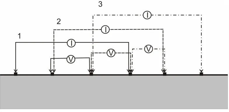
Figure 17 shows the way a multiple electrode array using Wenner geometry would be used to measure the resistivity of the top layer of the ground surface. If the array contains sufficient electrodes, the electrical properties at greater depths may be surveyed by using non-adjacent electrodes, which is equivalent to increasing the electrode spacing.

The overlapping measurements of multiple electrode arrays increase reliability of results. Reliability of the resistivities is least at the edges where resistivity values may rely on one measured value; subsequent analysis may produce edge effects in the resulting cross-sectional profile. Similarly, the reliability and resolution of resistivities is highest at the surface as deeper levels of resistivity will not have as many “overlapping” readings.

The apparent resistivity data can be converted into resistivity values using a mathematical inversion. The subsurface is divided into a number of rectangular blocks related to the electrode array configuration. A value of resistivity is assigned to each block to create a model of the subsurface that could result in the apparent resistivity values obtained during data collection and a profile of modelled resistivity is built up to create a “psuedosection”. The profile of the modelled resistivity is called a psuedosection as it represents a theoretical model of the possible true resistivity values which would create the apparent resistivity measured at the surface. The mathematical inversion does not have a unique solution (Geotomo software, 2004).

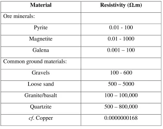
With the exception of metallic bodies most ground materials have low conductivities (and therefore high resistivities) meaning that they impede the flow of electrons within their structure. Table 2 shows a comparison of resistive and conductive common subsurface materials.

Table 2 Table of common resistivity values (from Milsom 2002)

Material Resistivity (Ω.m)

Ore minerals:

Pyrite 0.01 - 100

Magnetite 0.01 - 1000

Galena 0.001 – 100

Common ground materials:

Gravels 100 - 600

Loose sand 500 – 5000

Granite/basalt 100 – 100,000

Quartzite 500 – 800,000

cf. Copper 0.0000000168

3.4 Electromagnetism (EM):

Figure 18: Electromagnetic generation of a secondary magnetic field using a primary magnetic field generated from current travelling through a conductive loop. The secondary magnetic field then generates a measurable current in the receiver loop which is recorded.

currents in turn generate a secondary magnetic field that induces a current in the receiver loop at the surface.

Figure 19: A possible secondary EM response showing a rotation in Phase with Quadrature and real components.

Maxwell’s equations describe how the electromagnetic response is generated and the relationships between the strength of the magnetic field and magnitude of the induced current (conductivity) within the subsurface (Haliday et al. 2002). In general the more conductive a body is, the stronger the secondary magnetic field, as stronger electric currents are generated.

For high conductivities; penetration of signal using EM methods is often related to a “skin depth” which is the reciprocal of the attenuation constant (α refer previous) so that:

Skin depth = 1/ α

In areas of low conductivities the depth of penetration of EM methods is roughly proportional to the loop separation so that:

4: Methodology:

4.1 General survey set up:

After identification of the target ice wedge polygon, four corners for the survey area were chosen and fixed using an optical square. Survey areas were oriented so that surveys requiring sequential lines would run roughly north-south. Line spacing refers to the common offset of these north-south lines along the east-west baseline.

GPS measurements of the location of each corner were taken at least twice over the course of a day to reduce error associated with low satellite coverage of a location. The satellite coverage in Antarctica is not optimal for GPS accuracy as it needs both numerous satellites and for them to be spread out across the sky. This inaccuracy was seen best in the elevation data which could vary by up to as much as 20m for one location.

Electromagnetism and GPR surveys were conducted over the entire polygon area, while electrical resistivity surveys were conducted as cross-sectional lines through the polygon and over features of interest.

4.1.1 Factors involved in working in the Dry Valleys:

The cold weather and rough terrain found within the Dry Valleys effects the efficiency of collecting geophysical data. Batteries used to power resistivity and GPR antennas and consoles as well as the EM31 laptop, held less capacity than they would have in temperate conditions. For the best use of our time in the field additional planning was needed so that battery shortages would not cause a delay in the work schedule.

The cold conditions affected the fibre optic cables used in GPR by making them brittle and prone to breakages. In particular the casing surrounding the fibre-optic cables was very sensitive to breakages in the cold and had to be monitored carefully. For resistivity, the relative battery power and time required to run resistivity surveys was such that 3D geometries were not practical in the Dry Valleys during our field season.

Due to the delicate nature of the Dry Valleys environment and the relative difficulty of trenching or drilling in glacial diamict material no ground truth measurements were obtained to correlate this data.

Appendix 1 is a modified logistics report collated for K054’s field season in the Dry Valleys. The timeline for the data collection is outlined and the number of days required to complete each survey can be used as a guide for further research. Bad weather delays were minimal but injury to a party member caused re-assessment of the work achievable. Logistics issues surrounding the use of geophysical equipment are also noted there.

4.2 Topographic correction data:

One of the causes of error within geophysical methods is a lack of topographic correction which allows for the geophysical response to be corrected for variations in mass due to topography or displacement of reflected responses. The most detailed geophysical survey that was conducted as part of this project was the GPR with a line spacing of 0.5 m with the 200 MHz and 100 MHz surveys being offset by 0.25 m. For topographic measurements to run along each GPR line a 0.25 m grid was needed. This grid density was used for VVP2 but soon proved to be too labour intensive to be applied in Beacon Valley. As a result Beacon Valley topographic data was collected at 0.5 m x 0.5 m data density which corresponded to the 100 MHz and EM31 survey grid.

as the program for processing this information is capable of inferring the missing values and the benefits of such high data density had to be weighed against the time constraints.

Resistivity surveys extended past the limitations of the GPR grid and additional topographic measurements were taken at each electrode along the North-South and East-West strings.

4.2.1 Data collection:

Using an optical level and staff, measurements were taken from a standard datum level above the polygon surface (Figure 20). The tripod for the optical level was set up outside the survey area and used to measure the points along the survey grid.

GPS elevation measurements were taken at the base of the optical level tri-pod (X on Figure 20) and used to correct staff measurements to topography in m ASL (above sea level)

As the topography on VVP1 was limited to relief of less than 0.3m it was decided that the topographic corrections were of minor importance due to minimal effect on the placement of reflectors within the profiles

4.2.2 Data processing:

To correct the topographic staff measurements to elevation ASL the GPS elevation measurement from the base of the optical level (X on Figure 17) was added to the measured tripod height. Staff measurements were subtracted from the corrected elevation value using the equation line tool in Microsoft Excel. 200 MHz GPR lines were offset 0.25 m from the 0.5 m topographic grid. The averages of the topographic data from the lines of either side were taken to give approximate values. Data was sorted into the correct format for graphical gridding program (Surfer8) and used to

create topographic surfaces to record morphology and geometry. Individual line topographic data sets were saved in the form of a tab delimited ASCII file of “.TOP” file extension for topographically correcting GPR. Resistivity topography measurements were plotted as X-Y graphs showing topography features along the line and used to topographically correct modelled profiles.

4.3 Ground Penetrating Radar:

GPR data was collected using the pulseEKKO sensors and software 100A system using 50, 100 and 200 MHz antennas. The 50 MHz antennas were used for cross-sections through the surveyed polygon area, while the 100 and 200 MHz antennas were used for lines within the survey areas on 0.5m line spacing across the area to be merged for three dimensional analyses.

4.3.1 Data collection:

A CMP was conducted in Victoria Valley over VVP1 and along a cross valley transect line (Bannister, unpublished 2007). The CMP analysis was used to determine a subsurface velocity used in migrating the GPR data, discussed in data processing. All of the GPR PPG survey areas were covered using a reflection survey in step mode where each antenna is moved and placed a set distance from the last measurement. Step surveying was used because of the rough terrain where the placement of antennas would provide greater accuracy.

movements and increase the efficiency of the GPR, the survey lines for the 100 and 200 MHz antennas were run with a 0.25 m offset between them (refer Figure 21 for the resulting geometry). This methodology was applied to all of the polygonal areas surveyed in Victoria and Beacon Valley.

Figure 22 shows the components of the GPR system and images of the GPR data collection from Victoria and Beacon Valley.

3D GPR data is collected in multiple lines covering the entire area. Grasmuek et al. (2005) examines the data density required to fully resolve subsurface features with GPR and concludes that full GPR resolution can only be achieved with line spacing being equal to 2 times the step size. For working in 3D in the Dry Valleys this would have resulted in a line spacing of 0.2 m for the 200 MHz which was not practical for completion of the surveys in the given time. However, the line spacing of 0.5 m for 100 MHz is close to the 0.4 m requirement and so can be classified as full resolution 3D GPR. Data density is still greater in the south – north orientation than in the west – east orientation.

Antennas were separated by 2m for 50 MHz antenna GPR lines, 1 m for 100 MHz and 0.6 m for 200 MHz, as recommended by sensors and software pulseEKKO guidelines (Annan and Cosway, 1992) To avoid sampling errors, we applied a 0.5 m step size for the 50 MHz, 0.2 m step size for the 100 MHz and a 0.1 m step size for the 200 MHz antennas. Trace positions along the line are the position of the midpoint between the two antennas.

4.3.2 Data Processing

GPR data was processed using Sensors & Software pulseEKKO 4.2 for filtering migration and topographic corrections. EKKO3D and T3D were used for 3D merger and examination of the 3D data set. For consistency and to work within time constraints batch file processing was used for the 3D GPR data sets. Appendix 3 shows the GPR trace lines at raw, topographically corrected, and fully migrated stages of processing and the resulting 3D volumes.

CMP analysis:

Figure 23: CMP semblance analysis showing a plot of velocity measurements from within the subsurface of VVP1. In both a) and b) the highest concentration of velocities interpreted from the subsurface response is outlined by the box and is seen between 0.12 – 0.14 m/ns.

Topographic corrections:

The topography in these surveys effected the placement of the reflectors within the GPR line profiles. To correct the placement of reflectors to correct relative locations the topographic data collected (appendix 2) was applied to the GPR data using topographic addition where the trace profile is distorted to show the topographic effects, and topographically shifted where the reflector positions are repositioned using the topographic information and the subsurface velocity (determined by CMP).

Migration:

To collapse diffraction curves and position reflectors correctly within the profile. Two types of migration were used; mathematical Fourier transform migration in the frequency wave number domain (F-K) (refer to Stolt 1978 for details of this methodology), and synthetic aperture migration where a width of window has a conical filter applied to collapse diffraction curves. F-K migration was applied in batch file form while synthetic aperture migration was applied during merger into 3D cubes.

Filters:

To reduce the “wow” of the signal where ---- is amplified and distorts the response a “dewow” filter was applied whereby the low frequencies were removed from the traces.

Gain functions:

To correct for the loss of signal with depth due to signal attenuation; two types of gain functions were applied to these data sets; AGC and SEC gains.

reflectors across a profile but are less useful when evaluating signal response type and quality.

• SEC (Spreading and Exponential Compensation) is a limited exponential function where a limited gain inversely related to signal strength is applied (Annan 1993). The limited function allows weaker signals to be boosted but not to the point where relative signal strength relationships are filtered out. Late responses associated with greater depth are boosted but not to the level seen with an AGC gain, and weaker signals within the main body of the signal response maintain their correct relative signal strength.

4.3 3 Data display:

The GPR data in this thesis is displayed in Variable Area Display (VAD) greyscale with phase of GPR signal being represented by black for positive amplitude and white for negative amplitude. Large amplitude of signal from strong reflectors will produce strong signal patterns of black and white. Figure 30.

The relative phase of a reflector can indicate specific changes in the physical properties. The Airwave and groundwave have a - + - amplitude phase (refer profile lines Appendix IV). A strong reflector with a change in phase can indicate that the reflector represents a change into a medium of higher dielectric conductivity.

GPR data is presented in individual profile format (Refer to Appendix IV for full record of all profile lines collected for this thesis) and merged into 3D cubes using EKKO 3D

4.3 Resistivity:

Electrical imaging in the form of resistivity surveys were conducted in cross-sectional positions across the four surveyed polygonal ground sets and was the only method used that required any subsurface disturbance due to the penetration of electrodes to maintain electrical contact with the ground. The positions of the cross-sectional lines of resistivity were roughly central but varied according to the specific geometry of the polygonal areas and according to features to be targeted.

4.3.1 Data collection

Resistivity data were collected using a Geotomo resistivity system and ImagerPro software. All surveys were conducted using the Wenner array configuration using 32/64 electrodes with 0.5 or 1 m electrode spacing. Figure 24 shows images of the resistivity data collection during our field season.

The Geotomo resistivity tomography system passes current through multi channel electrode cables connected to a central control unit. (Figure 24a). The multi channel electrode cables allow initial current and electrical response to be isolated and recorded separate from each other. The electrode cables make contact with the ground through metal spikes planted into the ground and clipped onto the cable (Figure 24b). To avoid induction of a secondary current within the subsurface (refer EM theory section for the physical principles of this phenomena) the electrode cables are positioned so that no loops of cable are created (Figure 24c, d, and e.). The electrode cables are also shielded to further reduce risk of an unwanted secondary response.

made establishing and maintaining electrical contact with the ground surface difficult. Resistivity surveys were not run unless contact resistance tests came back without errors.

Figures 25 – 28 illustrate the positioning of the resistivity lines over PPG topography. Topography maps made from topography data with low elevation to high elevation being represented by dark to light shading. Lines slicing through topography profile plots of resistivity lines represent the GPR and EM survey area extent.

4.3.1.1 VVP1:

Once set up, the resistivity surveys were conducted as time lapse over VVP1. VVP1 was chosen for the intersecting contraction crack at its centre. Four resistivity lines were set up crossing through the central crack intersection (Figure 25) at right angles to each other running North – South and West – East respectively. The surveys were conducted using 32 electrodes at 1 m electrode spacing.

Electrodes were left in their positions in the ground for the duration of the time-lapse survey and resistivity lines were run every 4 days.

4.3.1.2 VVP2:

Three cross-sectional lines were conducted on VVP2; one Sorth – Nouth bisecting the long axis of the polygon and two running West – East offset from each other each centred on opposing contraction cracks (refer Figure 26). The surveys were set up using 32 electrodes and 0.5m electrode spacing for the West – East lines and 1 m spacing for the South – North line

4.3.1.3 BVP1: