Improved classi cation for compositional data using the $\alpha$ transformation

Munich Personal RePEc Archive

Improved classi cation for compositional

data using the

α

-transformation

Tsagris, Michail and Preston, Simon and T.A. Wood,

Andrew

Department of computer science, University of Crete, Heraklion,

Greece, School of Mathematical Sciences, University of Nottingham,

UK, School of Mathematical Sciences, University of Nottingham, UK

2016

Online at

https://mpra.ub.uni-muenchen.de/67657/

Improved classification for compositional data using the

α

_{-transformation}

Michail Tsagris1

, Simon Preston2

and Andrew T.A. Wood2 1

Department of computer science, University of Crete, Heraklion, Greece

2

School of Mathematical Sciences, University of Nottingham, UK

[email protected], [email protected] and [email protected]

Abstract

In compositional data analysis an observation is a vector containing non-negative values, only the relative sizes of which are considered to be of interest. Without loss of generality, a com-positional vector can be taken to be a vector of proportions that sum to one. Data of this type arise in many areas including geology, archaeology, biology, economics and political science. In this paper we investigate methods for classification of compositional data. Our approach centres on the idea of using theα-transformation to transform the data and then to classify the transformed data via regularised discriminant analysis and thek-nearest neighbours algorithm. Using theα-transformation generalises two rival approaches in compositional data analysis, one (when α=1) that treats the data as though they were Euclidean, ignoring the compositional constraint, and another (when α = 0) that employs Aitchison’s centred log-ratio transforma-tion. A numerical study with several real datasets shows that whether using α = 1 or α = 0 gives better classification performance depends on the dataset, and moreover that using an in-termediate value of α can sometimes give better performance than using either 1 or 0.

Keywords: compositional data, classification, α-transformation, α-metric, Jensen-Shannon divergence

1

Introduction

Compositional data arise commonly in many fields, for instance geology (Aitchison, 1982), in studying constitution of rock samples; economics (Fry et al., 2000), in budget allocations; archaeology (Baxter et al., 2005), in the constitution of man-made glasses; and the political sciences (Rodriques and Lima, 2009), in voting behaviour. In compositional data analysis, a composition is considered an equivalence class comprising the set of multivariate vectors that differ only by a scalar factor and have non-negative components. Consequently, without loss of generality, an observation may be viewed as a vector of proportions, i.e., with non-negative components constrained to sum to 1. The sample space of the observations is hence the simplex

Sd₌ (

(x1, ..., xD)T

xi≥0, D

X

i=1

xi = 1

)

,

whereD denotes the number of components of the vector andd=D−1.

(EDA) (Baxter, 2001; Baxter et al., 2005; Baxter and Freestone, 2006; Woronow, 1997). There is a school of thought, however, largely following from the work of Aitchison (1982, 1983, 1992), that ignoring the compositional constraint is inappropriate and can lead to misleading infer-ences. Aitchison contended that data should instead be analysed after applying a “logratio” transformation, arguing that this amounted to working with an implied distance measure on the simplex (discussed further in the next section) that satisfied particular mathematical properties he regarded as essential for compositional data analysis. Other approaches to compositional data analysis that we mention here but do not consider further in this paper include using differ-ent transformations, such as the square-root transformation (Stephens, 1982; Scealy and Welsh, 2011), and parametric modelling, for example using the Dirichlet distribution (Gueorguieva et al., 2008).

Both EDA and Aitchison’s logratio analysis (LRA) approach are widely used and there has been a long and ongoing disagreement over which of these approaches, or indeed others, is most appropriate to use. The debate remains largely centred on the distance measures implied by the various approaches and whether or not they satisfy particular mathematical properties. Scealy and Welsh (2014) have recently presented a historical summary of the debate, and have given a critical appraisal of the properties often invoked by authors to support the use of LRA. We share Scealy and Welsh’s opinion that LRA should not be a default choice for compositional data analysis on account of such properties. In this paper, we take the pragmatic view, which seems especially relevant for classification problems (in which out-of-sample classification error rate provides an objective measure of performance), that we should adopt whichever approach performs best in a given setting.

Indeed, a key message of this paper is that for classification problems, the choice of whether or not one should transform the data, and if so which transformation to use, should depend on the dataset under study. This conclusion is clear from the fact that we can easily generate a synthetic dataset for which LRA will perform perfectly and EDA poorly, and vice versa.

One characteristic of a dataset that immediately rules out using LRA in its standard form is the presence of observations for which one or more components is zero, since for such obser-vations the logratio transformation is undefined. Data of this type are not uncommon (in§4 we consider two datasets containing observations with zeros), so this is a notable weakness of LRA. Some attempts have been made to modify LRA to make it appropriate for data containing zeros (particularly when the zeros are assumed to arise from rounding error), but these involve a somewhat ad hoc imputation approach of replacing zeros with small values. On a different tack, Butler and Glasbey (2008) developed parametric models specifically for compositional data with zeros.

data as a basis for classification. This transformation has a free parameter,α, and is such that the case α = 0 corresponds to the logratio transformation, and α = 1 corresponds to a linear transformation of the data. Hence using α= 0 corresponds to LRA, and α= 1, when used in conjunction with the discriminant analysis and nearest-neighbour classification algorithms that we consider in§3, is equivalent to EDA. For values of αbetween 0 and 1, the α-transformation offers a compromise between LRA and EDA. An important benefit of the α-transformation is that it is well-defined for any α >0 for compositions containing zeros.

The paper is structured as follows. In§2 we discuss in more detail theα-transformation and the logratio transformation, and the associated implied distance measures, and then in §3 we consider some classification techniques and how their performance can be improved using the α-transformation. In §4 we present the results of a numerical study with four real datasets to investigate the performance of the various techniques. We conclude in §5 with a discussion of the results.

2

The

α

_{-transformation and implied simplicial distance}

mea-sure

The α-transformation of a compositional vectorx∈Sd _{(see Tsagris et al. (2011)) is defined by}

zα(x) =H·

Duα(x)−1D

α

, (1)

withα >0 (we discuss more generalα below), and where

uα(x) =

xα1

PD

j=1xαj

, . . . , x

α D

PD

j=1xαj

!T

(2)

is the compositional power transformation (Aitchison, 2003),1D is theD-dimensional vector of

ones, and His any d-by-Dmatrix consisting of orthonormal rows, each of which is orthogonal to1D; similar ideas have been used in the compositional data context by Egozque et al. (2003)

and, of course, in many other contexts. A suitable choice for H (noting in any case that the classification methods in this paper are invariant to the particular choice) is the Helmert matrix (Lancaster, 1965; Dryden and Mardia, 1998) with the first row removed, i.e., the matrix whose jth row is

(hj, . . . , hj,−jhj,0, . . . ,0), where hj =− {j(j+ 1)}

−1/2

, (3)

with hj repeated j times and 0 repeated d−j times. The purpose of H is to remove the

redundant dimension which is present due to the compositional constraint. In particular, the vector (Duα(x)−1D)/αhas components which sum to zero and therefore it lies in a subspace

ofRD_{; left-multiplication byHis an isometric one-to-one mapping from this subspace into}Rd_.

The image Vα =

zα(x) :x∈Sd of transformation (1) is Rd in the limit α → 0 but a strict

subset of Rd_{forα6= 0. Transformation (1) is invertible: for v∈ Vα the inverse ofzα(x) is}

z_α−1(v) =u_α−1αH⊤v+1D

where

u−_α1(x) = x

1/α

1

PD

j=1x 1/α j

, . . . , x

1_/α

D

PD

j=1x 1/α j

!

. (5)

If one is willing to exclude from the sample space the boundary of the simplex, which corresponds to observations that have one or more components equal to zero, then theα-transformation (1) and its inverse (4) are well defined for allα∈R_{. (Excluding the boundary is standard practise}

in LRA because the definition is used to sidestep the problem of having data with zeros.) The motivation for transformation (1) is that the case α = 0 corresponds to LRA, whereas α = 1 corresponds to EDA. We define the case α= 0 in terms of the limitα→0; then

z0(x) = lim

α→0zα(x) =H·w(x), (6)

where

w(x) =

log

x1

g(x)

, . . . ,log

xD

g(x)

T

, (7)

is Aitchison’s centred logratio transformation (Aitchison, 1983, 2003) and g(x) =QD

i=1x 1_/D

i is

the geometric mean of the components of x. See the Appendix for proof of (6). For the case α= 1, (1) is just a linear transformation of the simplex.

Power transformations similar to (1) were considered by Greenacre (2009) and Greenacre (2011), in the somewhat different context of correspondence analysis. A Box–Cox transforma-tion applied to each component ofx∈Sd _{so thatx is transformed to}

θ−1xθ1−1

, . . . , θ−1xθ_D−1T, (8)

has the limit (logx1, . . . ,logxD)T asθ→0. We favour transformation (1) in this work in view

of its closer connection, via (6), to Aitchison’s centred logratio transformation.

Theα-transformation (1) leads to a natural simplicial distance measure ∆α(x,y), which we

call the α-metric, between observations x,y ∈ Sd_{, defined in terms of the Euclidean distance}

k · k between transformed observations, i.e.,

∆α(x,y) =kzα(x)−zα(y)k

= D

|α|

  D X i=1 xα i PD

j=1xαj

− y

α i

PD

j=1yjα

!2 

1_/2

. (9)

The special case

∆0(x,y) := lim

α→0∆α(x,y) =

" _D X

i=1

log xi

g(x) −log yi

g(y)

2#

1_/2

is Aitchison’s distance measure (Aitchison et al., 2000), whereas

∆1(x,y) =D

" _D X

i=1

(xi−yi)

2

#1/2

(11)

is just Euclidean distance multiplied by D.

Transformation (1), and the implied distance measure (9), offer flexibility in data analysis: the choice ofαenables either LRA or EDA, or a compromise between the two, and the particular value ofα can be chosen to optimise some measure of practical performance (in this paper, the out-of-sample classification error rate). Crucially, for α > 0, the transformation and distance are well defined even when some components have zero values, in contrast to (7) and (10).

Amongst the criteria for compositional distance measures listed by Aitchison (1992), the distance measure (9) satisfies “positivity” (∆α(x,y)>0 forx6=y), “zero difference for

equiva-lent compositions” (∆α(x,x) = 0), “interchangeability of compositions” (∆α(x,y) = ∆α(y,x)),

“scale invariance” (∆α(ax, Ay) = ∆α(x,y) for alla >0, A >0) and “permutation invariance”

(∆α(Px, Py) = ∆α(x,y) for any permutationP). It does not satisfy “perturbation invariance”,

a property strongly tied to the logratio transformation (Aitchison, 2003); and nor does it sat-isfy “subcompositional coherence”, a criterion that affects inferences regarding the relationships between compositional components (Greenacre, 2011). The question of how much importance should be given to subcompositional coherence in compositional data analysis has been a matter of much debate; see for example the historical review and discussion in Scealy and Welsh (2014). Our view is similar to that of Scealy and Welsh (2014), which is that subcompositional domi-nance is not a property of primary importance, although we point out that a referee strongly disagrees with our position. We reiterate that our motivation is to achieve strong practical performance, whether or not our distance measure satisfies any particular properties.

3

Classification techniques for compositional data

The key idea now is to use the α-transformation (1) in conjunction with regularised descrim-inant analysis (RDA), and the α-metric (9) in conjunction with k-nearest-neighbours (k-NN) classification, to investigate how performance for various values ofα compares with the special cases of EDA (α = 1) and LRA (α = 0). We will begin with a brief review of regularised discriminant analysis, of which linear and quadratic discriminant analysis are special cases, and with thek-nearest neighbours algorithm.

3.1 Regularised discriminant analysis (RDA)

In discriminant analysis we allocate an observation to the group with the highest (posterior) density, assuming that observations in each group come from a multivariate normal distribu-tion. Given a training sample with g groups containing n1, . . . , ng observations, then a new

observation z ∈Rd _{is classified to the group for which the discriminant score,δi(z), is largest,}

where

δi(z) =−

1 2log

2π

ˆ

Σi

−

1

2(z−µˆi)

T_Σˆ−1

here | · | denotes determinant, πi =ni/nwith n=Pgi=1ni, and the ˆµi and ˆΣi are the sample

mean vector and covariance matrix, respectively, of theith group. Equation (12) is the Bayesian version of discriminant analysis, incorporating the prior group membership probabilities π =

(π1, . . . , πg), which assumes that the proportions of observations in the training sample are

representative of the proportions in the population. Other choices ofπ are possible depending

on available prior information. The frequentist version uses instead πi = 1/g. We will use the

Bayesian version withπi=ni/n in our numerical investigations in §4.

The boundary between classification regions, say between groups i and j, is defined by δi(z) =δj(z). From (12), the boundaries are hence quadratic in z, and for this reason the

ap-proach is termed quadratic discriminant analysis (QDA). If we make the simplifying assumption that the groups share a common covariance matrix, then the ˆΣi in (12) can be replaced with

the pooled estimate

ˆ

Σp =

Pg

i=1(ni−1) ˆΣi

n−g .

In this case, the boundaries are linear, and the approach is hence termed linear discriminant analysis (LDA).

QDA and LDA are special cases of so-called regularised discriminant analysis (RDA); see Hastie et al. (2001, pp. 112-113). The idea of RDA is to regularise the covariance matrices by replacing them with weighted averages

ˆ

Σi(λ, γ) = λΣˆi+ (1−λ) ˆΣp(γ),

and Σˆp(γ) = γΣˆp+ (1−γ) tr

ˆ

Σp

I/d, (13)

where λ, γ ∈ [0,1] are two free parameters and I is the d-by-d identity matrix. Parameter λ offers a trade-off between the more flexibile classification boundaries of QDA and the greater stability of LDA to one or more of the ˆΣi being ill-conditioned. Parameter γ offers further

stability if the pooled estimate ˆΣp is itself ill-conditioned. Choosingλ= 1 gives QDA, whereas

choosingλ= 0 andγ = 1 gives LDA.

We propose to use RDA with data transformed using the α-transformation (1), and will denote this by RDA(α, λ, γ). Hence, RDA(0, λ, γ) amounts to the LRA approach of applying RDA to data transformed using the isometric log-ratio transformation (6), whereas RDA(1, λ, γ) amounts to the EDA approach of applying RDA to untransformed data. We will also use the notation QDA(α) = RDA(α,1,0) and LDA(α) = RDA(α,0,1).

3.2 k_{-nearest neighbours (}k_-NN)

The k-NN algorithm is an intuitive classifier that assumes no parametric model. It involves determining thekobservations in the training sample that are closest, by some choice of distance measures, to the new test observation, then allocating the test observation to the group most common amongst these k “nearest neighbours”. Ties caused by two or more groups jointly being most common can be broken by allocating uniformly at random amongst the tied groups (the strategy we use in our numerical examples in§4) or else by using a secondary tie-breaking criterion.

which are flexible but which have a tendency to overfit, with the opposites true whenkis large. It also depends on the choice of distance measure. Since we are dealing with compositional data we shall use the α-metric (9), denoting such an approach k-NN(α), so k-NN(0) indicates the LRA approach of usingk-NN with Aitchison’s distance (10), whilek-NN(1) indicates the EDA approach of usingk-NN based on Euclidean distance.

We can equally easily use any of many other possible distance measures. For sake of com-paring performance with the α-metric we also consider one alternative, namely the following variant of the Jensen-Shannon divergence:

ESOV(x,y) =

v u u t

D

X

i=1

xilog

2xi

xi+yi

+yilog

2yi

xi+yi

. (14)

We use the notation ESOV after Endres and Schindelin (2003) and ¨Osterreicher and Vajda (2003) who independently proved that (14) satisfies the triangle inequality and thus is a metric. As with the α-metric (9), the ESOV metric (14) is well defined even when zero values are present. We denote thek-NN classifier based on metric (14) by k-NNESOV.

4

Applications of compositional classification

We will show four examples of applications of the proposed compositional discrimination tech-niques. In all cases we used real data sets, two of them having observations with zero values in some of the components, and the other two data sets having no zero values. The two bench-marks for comparison will be whenα= 0, which results in LRA, and whenα= 1, which results in EDA.

We performed RDA(α, λ, γ), k-NN(α), varying α in steps of 0.05 between -1 and 1 for datasets without zeros and between 0.05 and 1 for datasets with zeros (since in such circum-stances the α-transformation and α-metric are not defined for α ≤0), and varying the values of λandγ in steps of 0.1 between 0 and 1.

To estimate the rate of correct classification in out-of-sample prediction we used cross vali-dation. This involves dividing the set ofnobservations into training and test sets of size ntrain

and ntest respectively, training the classifier on the training set, then evaluating its prediction

accuracy of the test set. In view of the samples having groups with quite variable numbers of observations we used stratified random sampling to ensure that the training sets were repre-sentative of the test sets, and to arrange that all groups were represented in the test set. In particular, we randomly divided the samples into training and test sets so that

ni

n ≈ ni,train

ntrain

≈ ni,test

ntest

,

where ni,ni,train and n_i,test are the sample sizes of the ith group in the full, training and test

samples, respectively. We then estimated the rate of correct classification by

q= c ntest

where c is the number of observations in the test set correctly classified and ntest is the test

sample size.

For each of the classifiers RDA(α, λ, γ) andk-NN(α), the steps can be summarised as follows

Step 1. Partition the sample into training and test sets using stratified random sampling.

Step 2. For each combination of values of the free parameters (α, λ, γ for RDA;α, k fork-NN(α); train the classifier on the training set.

Step 3. Apply the classifiers to the test set, and calculateq in (15).

Step 4. Repeat steps 1−3 a large number, sayB, times, then estimate the rate of correct classi-fication as the average of the qs in Step 3.

For the calculations in the following section we took B = 200 which gave estimates of the rate of correct classification with small standard errors at reasonable computational cost.

4.1 Examples

We will now introduce four datasets to investigate the performance of the supervised classi-fication techniques described in §3. The datasets come from different fields, namely ecology, forensic science, hydrochemistry and economics.

Example 1: Fatty acid signature data (contains zero values)

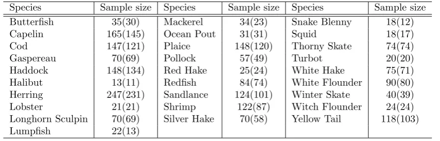
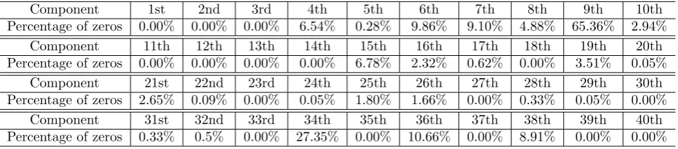
This is a dataset described in (Stewart and Field, 2011) (itself an updated version of a dataset from (Iverson et al., 2004)) which contains observations of n = 2110 fish of g = 28 different species, each observation being a composition with D= 40 components that characterises the fatty acid signature of the fish. A special feature of this dataset is that it contains many zero values (3506 components, across all observations, are zero) which rules out use of the log-ratio transformation (7). Table 1 shows the number of observations in each group, and the number of observations for which at least one component is zero. Table 2 shows the proportion of observations which have zeros in each of the components. For this example, for the cross validation we used a test set ofntest= 165 observations (7.8% of the full sample).

Species Sample size Species Sample size Species Sample size Butterfish 35(30) Mackerel 34(23) Snake Blenny 18(12) Capelin 165(145) Ocean Pout 31(31) Squid 18(17) Cod 147(121) Plaice 148(120) Thorny Skate 74(74) Gaspereau 70(69) Pollock 57(49) Turbot 20(20) Haddock 148(134) Red Hake 25(24) White Hake 75(71) Halibut 13(11) Redfish 84(74) White Flounder 90(80) Herring 247(231) Sandlance 124(101) Winter Skate 40(39) Lobster 21(21) Shrimp 122(87) Witch Flounder 24(24) Longhorn Sculpin 70(69) Silver Hake 70(58) Yellow Tail 118(103) Lumpfish 22(13)

Component 1st 2nd 3rd 4th 5th 6th 7th 8th 9th 10th Percentage of zeros 0.00% 0.00% 0.00% 6.54% 0.28% 9.86% 9.10% 4.88% 65.36% 2.94%

Component 11th 12th 13th 14th 15th 16th 17th 18th 19th 20th Percentage of zeros 0.00% 0.00% 0.00% 0.00% 6.78% 2.32% 0.62% 0.00% 3.51% 0.05%

Component 21st 22nd 23rd 24th 25th 26th 27th 28th 29th 30th Percentage of zeros 2.65% 0.09% 0.00% 0.05% 1.80% 1.66% 0.00% 0.33% 0.05% 0.00%

Component 31st 32nd 33rd 34th 35th 36th 37th 38th 39th 40th Percentage of zeros 0.33% 0.5% 0.00% 27.35% 0.00% 10.66% 0.00% 8.91% 0.00% 0.00%

Table 2: Fatty acid data: the percentage of observations for which each component is zero.

Example 2: Forensic glass data (contains zero values)

In the second example we use the forensic glass dataset (UC Irvine Machine Learning Repos-itory, 2014) which has n = 214 observations from g = 6 different categories of glass, where each observation is a composition with D = 8 components. The categories which occur are: containers (13 observations, 12 of which have at least one zero element), vehicle headlamps (29 observations, all with at least one zero value), tableware (9 observations, all with at least one zero value), vehicle window glass (17 observations, 16 with at least one zero value), window float glass (70 observations, 69 with at least one zero value) and window non-float glass (76 observations, 72 with at least one zero value). Once again the zeros rule out the use of LRA. In total there are 392 zero values; Table 3 shows in which components these zeros arise and Table 6 summarises the distribution of zeros across the observations. For the cross validation we used a test set consisted of ntest= 30 observations (14% of the total sample).

Components Sodium Magnesium Aluminium Silicon Percentage of zeros 0.00% 19.63% 0.00% 0.00% Components Potassium Calcium Barium Iron Percentage of zeros 14.02% 0.00% 82.24% 67.29%

Table 3: Forensic glass data: the percentage of observations for which each component is zero.

Example 3: Hydrochemical data (contains no zero values)

The hydrochemical data set (Otero et al., 2005) contains compositional observations onD= 14 chemicals (H, Na, K, Ca, Mg, Sr, Ba, NH4, Cl, HCO3, NO3, SO4, PO4, TOC) in water samples from tributaries of the Llobregat river in north-east Spain. Then= 485 observations are ing= 4 groups according to which tributary they were measured in: Anoia (143 observations), Cardener (95 observations), Upper Llobregat (135 observations) or Lower Llobregat (112 observations). For the cross validation in this example we used a training set of size ntest= 165 (34% of the

total sample size).

Example 4: National income data (contains no zero values)

in production assets, residential buildings, non-residential buildings, other buildings, and trans-portation equipment. The countries are categorised intog= 5 groups according to income levels and membership of the Organization for Economic Co-operation and Development (OECD); the groups are “low income” (10 countries), “lower middle income” (12 countries), “upper middle income” (9 countries), “high income and OECD member” (21 countries), and “high income and non-OECD member” (4 countries). For the cross validation, we used a test set of ntest = 10

observations (17.9% of the total sample).

4.2 Results

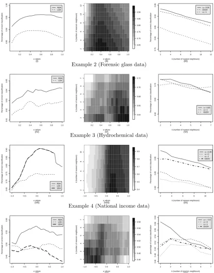
This section contains results from applying the methods of§3 to the four compositional datasets described above. Results are summarised in Figures 1 and 2 and Tables 4-7. The Tables show results for α= 1, α= 0, and for α free in [-1,1], in each case for the values of free parameters that maximise the estimated rate of correct classification.

Example 1 (Fatty acid signature data)

Estimated rate of Estimated rate of Method correct classification Method correct classification RDA(0.6,0.9,0.7) 0.962(0.014) RDA(1,0.8,1) 0.949(0.016)

LDA(0.45) 0.897(0.022) LDA(1) 0.868(0.024) 2-NN(0.35) 0.933(0.020) 2-NN(1) 0.849(0.027)

2-NNESOV 0.921(0.019)

Example 2 (Forensic glass data)

Estimated rate of Estimated rate of Method correct classification Method correct classification RDA(0.95,0.1,1) 0.643(0.034) RDA(1,0.1,1) 0.643(0.034)

LDA(0.4) 0.629(0.034) LDA(1) 0.629(0.034) 3-NN(0.85) 0.719(0.033) 2-NN(1) 0.719(0.033)

3-NNESOV 0.693(0.033)

Table 4: Estimated rate of correct classification of the different approaches. The standard error appears inside the parentheses.

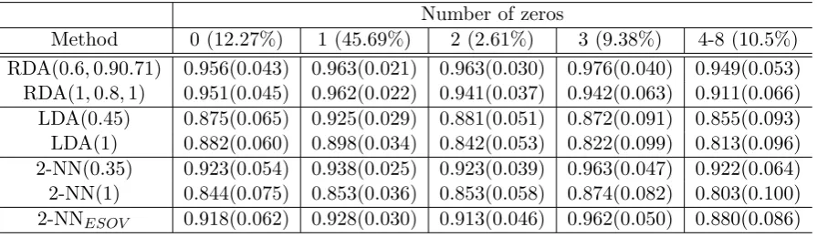
Number of zeros

Method 0 (12.27%) 1 (45.69%) 2 (2.61%) 3 (9.38%) 4-8 (10.5%) RDA(0.6,0.90.71) 0.956(0.043) 0.963(0.021) 0.963(0.030) 0.976(0.040) 0.949(0.053) RDA(1,0.8,1) 0.951(0.045) 0.962(0.022) 0.941(0.037) 0.942(0.063) 0.911(0.066) LDA(0.45) 0.875(0.065) 0.925(0.029) 0.881(0.051) 0.872(0.091) 0.855(0.093) LDA(1) 0.882(0.060) 0.898(0.034) 0.842(0.053) 0.822(0.099) 0.813(0.096) 2-NN(0.35) 0.923(0.054) 0.938(0.025) 0.923(0.039) 0.963(0.047) 0.922(0.064) 2-NN(1) 0.844(0.075) 0.853(0.036) 0.853(0.058) 0.874(0.082) 0.803(0.100) 2-NNESOV 0.918(0.062) 0.928(0.030) 0.913(0.046) 0.962(0.050) 0.880(0.086)

Example 1 (Fatty acid signature data)

0.2 0.4 0.6 0.8 1.0

0.85

0.90

0.95

1.00

(I)

α values

P

ercentage of correct classification

RDA LDA

0.2 0.4 0.6 0.8 1.0

2 4 6 8 10 12 (II)

α values

k (n

umber of nearest−neighbours)

0.65 0.70 0.75 0.80 0.85 0.90

2 4 6 8 10 12

0.75 0.80 0.85 0.90 0.95 (III)

k (number of nearest neighbours)

P

ercentage of correct classification

α =0.35 ESOV

α =1

Example 2 (Forensic glass data)

0.2 0.4 0.6 0.8 1.0

0.61 0.62 0.63 0.64 0.65 (IV)

α values

P

ercentage of correct classification

RDA LDA

0.2 0.4 0.6 0.8 1.0

2 3 4 5 6 7 (V)

α values

k (n

umber of nearest neighbours)

0.64 0.66 0.68 0.70 0.72

2 3 4 5 6 7

0.60

0.65

0.70

(VI)

k (number of nearest neighbours)

P

ercentage of correct classification

α =0.85

α =1 ESOV

Example 3 (Hydrochemical data)

−1.0 −0.5 0.0 0.5 1.0

0.65 0.70 0.75 0.80 0.85 0.90 (VII)

α values

P

ercentage of correct classification

RDA LDA QDA

−1.0 −0.5 0.0 0.5 1.0

2 4 6 8 10 (VIII)

α values

k (n

umber of nearest neighbours)

0.4 0.5 0.6 0.7 0.8 0.9

2 4 6 8 10

0.80

0.85

0.90

(IX)

k (number of nearest neighbours)

P

ercentage of correct classification

α =0.35

α =0

α =1 ESOV

Example 4 (National income data)

−1.0 −0.5 0.0 0.5 1.0

0.45

0.50

0.55

0.60

(X)

α values

P

ercentage of correct classification

RDA LDA QDA

−1.0 −0.5 0.0 0.5 1.0

2 3 4 5 6 7 (XI)

α values

k (n

umber of nearest−neighbours)

0.46 0.48 0.50 0.52 0.54 0.56 0.58

2 3 4 5 6 7

0.46 0.48 0.50 0.52 0.54 0.56 0.58 0.60 (XII)

k (number of nearest−neighbours)

percentage of correct classification

α = −0.5

α =0

α =1 ESOV

0.6 0.7 0.8 0.9 1.0

0.85

0.90

0.95

1.00

Proportion of zeros

Rate of correct classification

0.6 0.7 0.8 0.9 1.0

0.6

0.7

0.8

0.9

1.0

Proportion of zeros

Rate of correct classification

0.6 0.7 0.8 0.9 1.0

0.75

0.80

0.85

0.90

0.95

1.00

Proportion of zeros

Rate of correct classification

RDA(0.6,0.9,0.7) LDA(0.45) 2-NN(0.35)

Figure 2: Fatty acid signature data: the estimated rate of correct classification accuracy by group versus the the proportion of observations within the group that contain at least one zero.

Number of zeros

Method 0 (3.27%) 1 (29.44%) 2 (50.93%) 3 (13.55%) 4 (2.80%) RDA(0.95,0.1,1) 0.421(0.433) 0.582(0.173) 0.668(0.111) 0.787(0.233) 0.402(0.463)

RDA(1,0.1,1) 0.428(0.435) 0.585(0.174) 0.665(0.112) 0.788(0.233) 0.397(0.459) LDA(0.4) 0.404(0.431) 0.536(0.165) 0.636(0.120) 0.869(0.194) 0.689(0.412) LDA(1) 0.397(0.430) 0.523(0.162) 0.673(0.110) 0.790(0.230) 0.463(0.462) 3-NN(0.85) 0.307(0.394) 0.713(0.160) 0.717(0.108) 0.925(0.146) 0.387(0.429) 2-NN(1) 0.568(0.441) 0.715(0.160) 0.712(0.114) 0.870(0.178) 0.387(0.429) 3-NNESOV 0.477(0.447) 0.644(0.164) 0.764(0.097) 0.731(0.243) 0.387(0.429)

Table 6: Forensic glass data: classification accuracy by number of zeros. The estimated rate of correct classification is shown (with standard errors in parentheses).

Fatty acid and glass data from Examples 1 and 2

For both the fatty acid and forensic glass datasets, some of the groups have fewer observations than the dimensionDof the compositions, so QDA cannot be applied (since at least one of the

ˆ

Σi in (12) is singular). Both RDA, LDA andk-NN are applicable, however, and Table 4 shows

a comparison of performance for these techniques.

For the fatty acid data, RDA performs strongest, and best performance is achieved when α= 0.6. For this dataset k-NN(α) performs strongly too, withα = 0.35 giving notably better performance thanα= 1 (which corresponds to the EDA approach). For the forensic glass data, k-NN outperformed RDA and LDA, and the flexibility of having α different from 1 offered no improvement.

Example 3 (Hydrochemical data)

Estimated Estimated Estimated

Method rate of Method rate of Method rate of

correct correct correct

classification classification classification RDA(0.15,1,0) 0.909(0.02) RDA(0,1,0) 0.901(0.021) RDA(1,0.9,0.9) 0.793(0.029)

QDA(0.15) 0.909(0.02) QDA(0) 0.901(0.021) QDA(1) -LDA(0) 0.750(0.031) LDA(0) 0.750(0.031) LDA(1) -2-NN(0.25) 0.927(0.020) 2-NN(0) 0.855(0.026) 2-NN(1) 0.830(0.027) 3-NNESOV 0.899(0.021)

Example 4 (National income data)

Estimated Estimated Estimated

Method rate of Method rate of Method rate of

correct correct correct

classification classification classification RDA(−0.05,0.5,0) 0.574(0.035) RDA(0,0.5,0) 0.574(0.035) RDA(1,0.2,0) 0.540(0.035) QDA(−0.25) 0.496(0.035) QDA(0) 0.487(0.035) QDA(1) 0.431(0.035) LDA(0.5) 0.503(0.035) LDA(0) 0.488(0.035) LDA(1) 0.483(0.035) 2-NN(−0.5) 0.586(0.035) 3-NN(0) 0.533(0.035) 3-NN(1) 0.515(0.035)

3-NNESOV 0.541(0.035)

Table 7: Estimated rate of correct classification of the different approaches (with standard errors in parentheses).

classification accuracy and number of zeros. Corresponding results in Table 6 for the forensic glass data show lower classification accuracy for observations with 0 or 4 zeros compared with observations with 1, 2 or 3 zeros, albeit with large standard errors on account of the small number of such observations. Hence, again, the conclusion is that there is no clear evidence that zeros make observations any more or less difficult to classify correctly.

The key points from these examples are that LRA is not directly applicable because of the zeros, but EDA (α = 1) performs quite well with RDA having better performance in one example and k-NN in another, and in one of the examples letting α be a value other than 1 gave a further improvement.

Hydrochemical and national income data from Examples 3 and 4

For the hydrochemical data the extra flexibility of RDA over QDA offers no improvement (and hence RDA and QDA give identical results). Ill-conditioning of covariance matrices makes QDA and LDA unstable forα >0.75, which is why in Figure 1(VII) the lines corresponding to these methods stop at α = 0.75. The plots in the left column of Figure 1 show clearly that the performance of RDA(α, λ, γ) (and its special cases QDA(α) and LDA(α)) depends on α and tend to do best at values of α other than 0 or 1. k-NN(α) does best for this example, with α= 0.25 and 2 nearest neighbours, leading to the best performance of all the classifiers.

5

Conclusions

We have considered the α-transformation (1) and the α-metric (9) as a means to adapt LDA, QDA, RDA and k-NN for compositional data. This generalises EDA and LRA approaches via the parameter α, the choice of which enable a compromise between the two. Rather than choosing either EDA or LRA, our approach enables a choice ofα based on the dataset at hand, and numerical results suggest there is a clear benefit to having this flexibility.

An important benefit is that such an approach is well defined even when the dataset contains observations with components equal to zero, unlike with LRA in which ad hoc modifications to the data are needed prior to applying the log-ratio transformation. Within k-NN it is simple to incorporate any choice of distance that seems appropriate.

Appendix

Relationship between the α-transformation and centred log-ratio transformation

The proof that the transformation (Duα(x)−1D)/αdefined on the right-hand side of (1) tends

to the centred log-ratio transformation (7) asα →0 is as follows: for component i,

1 α

Dxα_i

PD

j=1xαj

−1 ! = D α  

1 +αlogxi+O α2

D1 +_Dα PD

j=1logxj +O(α 2₎−

1 D   =   

(1 +αlogxi)



1 +

α D

D

X

j=1

logxj





−1

−1 +O α2    . α =   

(1 +αlogxi)



1−

α D

D

X

j=1

logxj



−1 +O α

2    . α =   

1 +αlogxi−

α D

D

X

j=1

logxj−1 +O α2

   . α

= logxi−log D

Y

j=1

x1_j/D+O(α)

→ log

xi

g(x)

as α→0.

The proof that theα-metric (9) tends to the LRA metric (10) asα→0 follows from this proof.

References

AITCHISON, J. (1982), ”The statistical analysis of compositional data”, Journal of the Royal Statistical Society. Series B, 44, 139–177.

AITCHISON, J. (1983), ”Principal component analysis of compositional data”, Biometrika, 70,

AITCHISON, J. (1992), ”On criteria for measures of compositional difference”, Mathematical Geology, 24, 365–379.

AITCHISON, J. (2003), ”The Statistical Analysis of Compositional Data” (Reprinted with additional material by The Blackburn Press), London (UK): Chapman & Hall.

AITCHISON, J. and BARCELO-VIDAL, C. and MARTIN-FERNANDEZ, J.A. and PAWLOWSKY-GLAHN, V. (2000), ”Logratio analysis and compositional distance”, Math-ematical Geology, 32, 271–275.

BAXTER, M. J. (2001), ”Statistical modelling of artefact compositional data”, Archaeome-try, 43, 131–147.

BAXTER, M. J., BEARDAH, C. C., COOL, H. E. M., and JACKSON, C. M. (2005), ”Com-positional data analysis of some alkaline glasses”, Mathematical Geology, 37,183–196.

BAXTER, M. J. and FREESTONE, I. C. (2006), ”Log-ratio compositional data analysis in archaeometry”, Archaeometry, 48,511–531.

BUTLER, A. and GLASBEY, C. (2008), ”A latent Gaussian model for compositional data with zeros”, Journal of the Royal Statistical Society: Series C, 57,505–520.

DRDYEN, I. L. and MARDIA, K. V. (1998), ”Statistical Shape Analysis”, New York: Wiley.

EGOZQUE, J.J. and PAWLOWSKY-GLAHN, V. and MATEU-FIGUERAS, G. and BARCELO-VIDAL, C. (2003), ”Isometric logratio transformations for compositional data analysis”, Mathematical Geology, 35, 279–300.

ENDRES, D. M. and SCHINDELIN, J. E. (2003), ”A new metric for probability distributions”,

Information Theory, IEEE Transactions on, 49, 1858–1860.

FRY, J. M., FRY, T. R. L., and McLAREN, K. R. (2000), ”Compositional data analysis and zeros in micro data”, Applied Economics, 32,953–959.

GREENACRE, M. (2009), ”Power transformations in correspondence analysis”, Computational Statistics & Data Analysis, 53, 3107–3116.

GREENACRE, M. (2011), ”Measuring subcompositional incoherence”, Mathematical Geo-sciences, 43, 681–693.

GUEORGUIEVA, R., ROSENHECK, R., and ZELTERMAN, D. (2008), ”Dirichlet compo-nent regression and its applications to psychiatric data”, Computational statistics & data analysis, 52,5344–5355.

HASTIE, T., TIBSHIRANI, R., and FRIEDMAN, J. (2001), ”The Elements of Statistical Learning: Data Mining, Inference, and Prediction”, Berlin: Springer.

LANCASTER, H. O. (1965), ”The Helmert matrices”, American Mathematical Monthly, 72,

4–12.

LARROSA, J. M. (2003), ”A compositional statistical analysis of capital stock”, In Proceedings of the 1st Compositional Data Analysis Workshop, Girona, Spain.

NEOCLEOUS, T., AITKEN, C., and ZADORA, G. (2011), ”Transformations for compositional data with zeros with an application to forensic evidence evaluation”, Chemometrics and Intelligent Laboratory Systems, 109, 77–85.

OSTERREICHER, F. and VAJDA, I. (2003), ”A new class of metric divergences on probability spaces and its applicability in statistics”, Annals of the Institute of Statistical Mathemat-ics, 55, 639–653.

OTERO, N., TOLOSANA-DELGADO, R., SOLER, A., PAWLOWSKY-GLAHN, V., and CANALS, A. (2005), ”Relative vs. absolute statistical analysis of compositions: A com-parative study of surface waters of a mediterranean river”, Water Research, 39,1404–1414. PALAREA-ALBALADEJO, J., MARTIN-FERNANDEZ, J. A. and SOTO, J. A. (2012),

”Deal-ing with distances and transformations for fuzzy c-means cluster”Deal-ing of compositional data”,

Journal of classification, 29, 144–169.

RODRIGUES, P. C. and LIMA, A. T. (2009), ”Analysis of an European union election using principal component analysis”, Statistical Papers, 50, 895–904.

SCEALY, J. L. and WELSH, A. H. (2011), ”Regression for compositional data by using distri-butions defined on the hypersphere”, Journal of the Royal Statistical Society. Series B, 73,

351–375.

SCEALY, J. L. and WELSH, A. H. (2014), ”Colours and cocktails: compositional data analysis. 2013 Lancaster lecture”, Australian & New Zealand Journal of Statistics, 56,145–169. STEPHENS, M. A. (1982), ”Use of the von Mises distribution to analyse continuous

propor-tions”, Biometrika, 69, 197–203.

STEWART, C. and FIELD, C. (2011), ”Managing the essential zeros in quantitative fatty acid signature analysis”, Journal of Agricultural, Biological, and Environmental Statistics, 16,

45–69.

TSAGRIS, M. T., PRESTON, S., and WOOD, A. T. A. (2011), ”A data-based power trans-formation for compositional data”, In Proceedings of the 4th Compositional Data Analysis Workshop, Girona, Spain.

UC IRVINE MACHINE LEARNING REPOSITORY (2014), ”Forensic Glass Dataset”,

http://archive.ics.uci.edu/ml/datasets/Glass+Identification.

WORONOW, A. (1997), ”The elusive benefits of logratios”, In Proceedings of the 3rd Annual Conference of the International Association for Mathematical Geology, Barcelona, Spain. ZADORA, G., NEOCLEOUS, T., and AITKEN, C. (2010), ”A two-level model for evidence