Supervised Model Learning with Feature Grouping
based on a Discrete Constraint
Jun Suzuki and Masaaki Nagata
NTT Communication Science Laboratories, NTT Corporation 2-4 Hikaridai, Seika-cho, Soraku-gun, Kyoto, 619-0237 Japan {suzuki.jun, nagata.masaaki}@lab.ntt.co.jp
Abstract
This paper proposes a framework of super-vised model learning that realizes feature grouping to obtain lower complexity mod-els. The main idea of our method is to integrate a discrete constraint into model learning with the help of the dual decom-position technique. Experiments on two well-studied NLP tasks, dependency pars-ing and NER, demonstrate that our method can provide state-of-the-art performance even if the degrees of freedom in trained models are surprisingly small, i.e., 8 or even 2. This significant benefit enables us to provide compact model representation, which is especially useful in actual use.
1 Introduction
This paper focuses on the topic of supervised model learning, which is typically represented as the following form of the optimization problem:
ˆ
w= arg min
w
O(w;D) ,
O(w;D) =L(w;D) + Ω(w), (1) where Dis supervised training data that consists
of the corresponding inputx and output y pairs,
that is,(x,y)∈ D.wis anN-dimensional vector representation of a set of optimization variables, which are also interpreted as feature weights.
L(w;D)andΩ(w) represent a loss function and
a regularization term, respectively. Nowadays, we, in most cases, utilize a supervised learning method expressed as the above optimization problem to estimate the feature weights of many natural lan-guage processing (NLP) tasks, such as text clas-sification, POS-tagging, named entity recognition, dependency parsing, and semantic role labeling.
In the last decade, the L1-regularization tech-nique, which incorporates L1-norm into Ω(w),
has become popular and widely-used in many NLP tasks (Gao et al., 2007; Tsuruoka et al.,
2009). The reason is thatL1-regularizers encour-age feature weights to be zero as much as pos-sible in model learning, which makes the resul-tant model a sparse solution (many zero-weights exist). We can discard all features whose weight is zero from thetrained model1without any loss.
Therefore,L1-regularizers have the ability to eas-ily and automatically yieldcompactmodels with-out strong concern over feature selection.
Compact models generally have significant and clear advantages in practice: instances are faster loading speed to memory, less memory occupa-tion, and even faster decoding is possible if the model is small enough to be stored in cache mem-ory. Given this background, our aim is to establish a model learning framework that can reduce the model complexity beyond that possible by sim-ply apsim-plyingL1-regularizers. To achieve our goal, we focus on the recently developed concept of au-tomatic feature grouping (Tibshirani et al., 2005; Bondell and Reich, 2008). We introduce a model learning framework that achieves feature group-ing by incorporatgroup-ing a discrete constraint durgroup-ing model learning.
2 Feature Grouping Concept
Going beyond L1-regularized sparse modeling, the idea of ‘automatic feature grouping’ has re-cently been developed. Examples are fused lasso (Tibshirani et al., 2005), grouping pur-suit (Shen and Huang, 2010), and OSCAR (Bon-dell and Reich, 2008). The concept of automatic feature grouping is to find accurate models that have fewer degrees of freedom. This is equiva-lent to enforce every optimization variables to be equal as much as possible. A simple example is thatwˆ1= (0.1,0.5,0.1,0.5,0.1)is preferred over
ˆ
w2 = (0.1,0.3,0.2,0.5,0.3) since wˆ1 and wˆ2 have two and four unique values, respectively.
There are several merits to reducing the degree
1This paper refers to model after completion of
(super-vised) model learning as “trained model”
of freedom. For example, previous studies clari-fied that it can reduce the chance of over-fitting to the training data (Shen and Huang, 2010). This is an important property for many NLP tasks since they are often modeled with a high-dimensional feature space, and thus, the over-fitting problem is readily triggered. It has also been reported that it can improve the stability of selecting non-zero fea-tures beyond that possible with the standard L 1-regularizer given the existence of many highly cor-related features (J¨ornsten and Yu, 2003; Zou and Hastie, 2005). Moreover, it can dramatically re-duce model complexity. This is because we can merge all features whose feature weight values are equivalent in the trained model into a single fea-ture cluster without any loss.
3 Modeling with Feature Grouping
This section describes our proposal for obtaining a feature grouping solution.
3.1 Integration of a Discrete Constraint LetS be a finite set of discrete values, i.e., a set integer from−4to 4, that is,S={−4,. . .,−1,0, 1,. . .,4}. The detailed discussion how we define
S can be found in our experiments section since it deeply depends on training data. Then, we de-fine the objective that can simultaneously achieve a feature grouping and model learning as follows:
O(w;D) =L(w;D) + Ω(w)
s.t. w∈ SN. (2)
whereSN is the cartesian power of a setS. The only difference with Eq. 1 is the additional dis-crete constraint, namely, w ∈ SN. This
con-straint means that each variable (feature weight) in trained models must take a value in S, that is,
ˆ
wn ∈ S, where wˆn is then-th factor of wˆ, and n ∈ {1, . . . , N}. As a result, feature weights in trained models are automatically grouped in terms of the basis of model learning. This is the basic idea of feature grouping proposed in this paper.
However, a concern is how we can efficiently optimize Eq. 2 since it involves a NP-hard combi-natorial optimization problem. The time complex-ity of the direct optimization is exponential against N. Next section introduces a feasible algorithm.
3.2 Dual Decomposition Formulation
Hereafter, we strictly assume that L(w;D) and Ω(w) are both convex in w. Then, the
proper-ties of our method are unaffected by the selection
ofL(w;D)andΩ(w). Thus, we ignore their spe-cific definition in this section. Typical cases can be found in the experiments section. Then, we re-formulate Eq. 2 by using the dual decomposition technique (Everett, 1963):
O(w,u;D) =L(w;D) + Ω(w) + Υ(u)
s.t. w=u, andu∈ SN. (3)
Difference from Eq. 2, Eq. 3 has an additional term
Υ(u), which is similar to the regularizer Ω(w),
whose optimization variables wand u are
tight-ened with equality constraintw=u. Here, this paper only considers the caseΥ(u) = λ22 ||u||2
2+ λ1||u||1, and λ2 ≥ 0 andλ1 ≥ 02. This objec-tive can also be viewed as the decomposition of the standard loss minimization problem shown in Eq. 1 and the additional discrete constraint regu-larizer by the dual decomposition technique.
To solve the optimization in Eq. 3, we lever-age thealternating direction method of multiplier
(ADMM) (Gabay and Mercier, 1976; Boyd et al., 2011). ADMM provides a very efficient optimiza-tion framework for the problem in the dual decom-position form. Here, α represents dual variables for the equivalence constraintw=u. ADMM
in-troduces the augmented Lagrangian term ρ 2||w−
u||2
2 withρ >0which ensures strict convexity and increases robustness3.
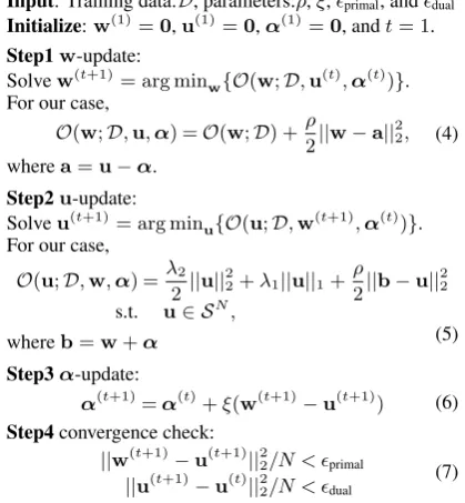
Finally, the optimization problem in Eq. 3 can be converted into a series of iterative optimiza-tion problems. Detailed derivaoptimiza-tion in the general case can be found in (Boyd et al., 2011). Fig. 1 shows the entire model learning framework of our proposed method. The remarkable point is that ADMM works by iteratively computing one of the three optimization variable setsw,u, andαwhile holding the other variables fixed in the iterations t= 1,2, . . .until convergence.
Step1 (w-update): This part of the
optimiza-tion problem shown in Eq. 4 is essentially Eq. 1 with a ‘biased’L2-regularizer. ‘bias’ means here that the direction of regularization is toward point
a instead of the origin. Note that it becomes a standard L2-regularizer if a=0. We can select any learning algorithm that can handle the L 2-regularizer for this part of the optimization.
Step2 (u-update):This part of the optimization
problem shown in Eq. 5 can be rewritten in the
2Note that this setting includes the use of onlyL1-,L2-,
or without regularizers (L1only:λ1>0andλ2= 0,L2only: λ1= 0andλ2>0, and without regularizer:λ1= 0, λ2= 0).
Input: Training data:D, parameters:ρ,ξ,primal, anddual
Initialize:w(1)=0,u(1)=0,α(1)=0, andt= 1.
Step1w-update: Solvew(t+1)= arg min
w{O(w;D,u(t),α(t))}.
For our case,
O(w;D,u,α) =O(w;D) +ρ
2||w−a||
2 2, (4) wherea=u−α.
Step2u-update:
Solveu(t+1)= arg minu{O(u;D,w(t+1),α(t))}.
For our case,
O(u;D,w,α) =λ2 2 ||u||
2
2+λ1||u||1+ρ
2||b−u||
2 2 s.t. u∈ SN,
(5) whereb=w+α
Step3α-update:
α(t+1)=α(t)+ξ(w(t+1)−u(t+1)) (6)
Step4convergence check:
||w(t+1)−u(t+1)||22/N < primal ||u(t+1)−u(t)||2
2/N < dual (7)
Break the loop if the above two conditions are reached, or go back to Step1 witht=t+ 1.
Output:u(t+1)
Figure 1: Entire learning framework of our method derived from ADMM (Boyd et al., 2011).
following equivalent simple form:
ˆ
u= arg minu{12||u−b0||22+λ01||u||1}
s.t. u∈ SN, (8)
where b0 = λ2+ρρ b, and λ01 = λ2λ1+ρ. This
optimization is still a combinatorial optimization problem. However unlike Eq. 2, this optimization can be efficiently solved.
Fig. 2 shows the procedure to obtain the exact
solution of Eq. 5, namelyu(t+1). The remarkable point is that the costly combinatorial optimization problem is disappeared, and instead, we are only required to perform two feature-wise calculations whose total time complexities isO(Nlog|S|)and
fully parallelizable. The similar technique has been introduced in Zhong and Kwok (2011) for discarding a costly combinatorial problem from the optimization with OSCAR-regularizers with the help of proximal gradient methods,i.e., (Beck and Teboulle, 2009).
[image:3.595.307.528.65.207.2]We omit to show the detailed derivation of Fig. 2 because of the space reason. However, this is easily understandable. The key properties are the following two folds; (i) The objective shown in Eq. 8 is a convex and also symmetric function with respect touˆ0, whereuˆ0is the optimal solution
of Eq. 8 without the discrete constraint. Therefore, the optimal solution uˆ is at the point where the
Input:b0= (b0n)Nn=1,λ01, andS.
1, Find the optimal solution of Eq. 8 without the constraint. The optimization of mixedL2 andL1-norms is known to have a closed form solution,i.e., (Beck and Teboulle, 2009), that is;
ˆ
u0n=sgn(b0n) max(0,|b0n| −λ01), where(ˆu0
n)Nn=1= ˆu0.
2, Find the nearest valid point inSNfromuˆ0in terms of the
L2-distance;
ˆ
un= arg min u∈S
(ˆu0n−u)2
where(ˆun)Nn=1= ˆu. This can be performed by a binary search, whose time complexity is generallyO(log|S|).
[image:3.595.75.285.67.294.2]Output:uˆ
Figure 2: Procedure for solving Step2
nearest valid point givenSN fromuˆ0 in terms of
theL2-distance. (ii) The valid points givenSNare always located at the vertexes ofaxis-aligned or-thotopes (hyperrectangles)in the parameter space of feature weights. Thus, the solutionuˆ, which is
the nearest valid point fromuˆ0, can be obtained by
individually taking the nearest value inS fromuˆ0n
for alln.
Step3 (α-update):We perform gradient ascent on dual variables to tighten the constraintw=u.
Note thatξ is the learning rate; we can simply set it to 1.0 for every iteration (Boyd et al., 2011).
Step4 (convergence check):It can be evaluated both primal and dual residuals as defined in Eq. 7 with suitably smallprimalanddual.
3.3 Online Learning
We can select an online learning algorithm for Step1 since the ADMM framework does not re-quire exact minimization of Eq. 4. In this case, we perform one-pass update through the data in each ADMM iteration (Duh et al., 2011). Note that the total calculation cost of our method does not in-crease much from original online learning algo-rithm since the calculation cost of Steps 2 through 4 is relatively much smaller than that of Step1.
4 Experiments
We conducted experiments on two well-studied NLP tasks, namely named entity recognition (NER) and dependency parsing (DEPAR).
Our decoding models are the Viterbi algorithm on CRF (Lafferty et al., 2001), and the second-order parsing model proposed by (Carreras, 2007) for NER and DEPAR, respectively. Features are automatically generated according to the defined feature templates widely-used in the pre-vious studies. We also integrated the cluster fea-tures obtained by the method explained in (Koo et al., 2008) as additional features for evaluating our method in the range of the current best systems.
Evaluation measures: The purpose of our ex-periments is to investigate the effectiveness of our proposed method in terms of both its performance and the complexity of the trained model. There-fore, our evaluation measures consist of two axes. Task performance was mainly evaluated in terms of the complete sentence accuracy (COMP) since the objective of all model learning methods eval-uated in our experiments is to maximize COMP. We also report the Fβ=1 score (F-sc) for NER, and the unlabeled attachment score (UAS) for DE-PAR for comparison with previous studies. Model complexity is evaluated by the number of non-zero active features (#nzF) and the degree of freedom (#DoF) (Zhong and Kwok, 2011). #nzF is the number of features whose corresponding feature weight is non-zero in the trained model, and #DoF is the number of unique non-zero feature weights. Baseline methods: Our main baseline is L 1-regularized sparse modeling. To cover both batch and online leaning, we selected L1-regularized CRF (L1CRF) (Lafferty et al., 2001) optimized by OWL-QN (Andrew and Gao, 2007) for the NER experiment, and the L1-regularized regularized
dual averaging (L1RDA) method (Xiao, 2010)4
for DEPAR. Additionally, we also evaluated L2-regularized CRF (L2CRF) with L-BFGS (Liu and Nocedal, 1989) for NER, and passive-aggressive algorithm (L2PA) (Crammer et al., 2006)5for
DE-PAR sinceL2-regularizer often provides better re-sults thanL1-regularizer (Gao et al., 2007).
For a fair comparison, we applied the proce-dure of Step2 as a simple quantization method to trained models obtained from L1-regularized model learning, which we refer to as (QT).
4RDA provided better results at least in our experiments
thanL1-regularized FOBOS (Duchi and Singer, 2009), and its variant (Tsuruoka et al., 2009), which are more familiar to the NLP community.
5L2PA is also known as a loss augmented variant of
one-best MIRA, well-known in DEPAR (McDonald et al., 2005).
4.1 Configurations of Our Method
Base learning algorithm: The settings of our method in our experiments imitateL1-regularized learning algorithm since the purpose of our experiments is to investigate the effectiveness against standard L1-regularized learning algo-rithms. Then, we have the following two possible settings; DC-ADMM: we leveraged the baseline L1-regularized learning algorithm to solve Step1, and set λ1 = 0 and λ2 = 0 for Step2. DCwL1-ADMM: we leveraged the baselineL2-regularized learning algorithm, but withoutL2-regularizer, to solve Step1, and setλ1>0andλ2= 0for Step2. The difference can be found in the objective func-tionO(w,u;D)shown in Eq. 3;
(DC-ADMM) : O(w,u;D) =L(w;D)+λ1||w||1
(DCwL1-ADMM) : O(w,u;D) =L(w;D)+λ1||u||1
In other words, DC-ADMM utilizes L1-regularizer as a part of base leaning algorithm
Ω(w) =λ1||w||1, while DCwL1-ADMM discards regularizer of base learning algorithmΩ(w), but
instead introducing Υ(u) = λ1||u||1. Note that these two configurations are essentially identical since objectives are identical, even though the formulation and algorithm is different. We only report results of DC-ADMM because of the space reason since the results of DCwL1-ADMM were nearly equivalent to those of DC-ADMM.
Definition ofS: DC-ADMM can utilize any
fi-nite set forS. However, we have to carefully se-lect it since it deeply affects the performance. Ac-tually, this is the most considerable point of our method. We preliminarily investigated the several settings. Here, we introduce an example of tem-plate which is suitable for large feature set. Let η,δ, andκrepresent non-negative real-value con-stants, ζ be a positive integer, σ ={−1,1}, and a function fη,δ,κ(x, y) =y(ηκx +δ). Then, we define a finite set of valuesSas follows:
Sη,δ,κ,ζ={fη,δ,κ(x, y)|(x, y)∈ Sζ×σ} ∪ {0}, where Sζ is a set of non-negative integers from zero toζ−1, that is,Sζ={m}ζm=0−1. For example, if we setη= 0.1, δ= 0.4,κ= 4, andζ= 3, then
81.0 83.0 85.0 87.0 89.0 91.0
1.0E+00 1.0E+03 1.0E+06 DC-ADMM L1CRF (w/ QT) L1CRF L2CRF
C
om
pl
et
e
S
ent
enc
e
A
cc
ur
ac
y quantized
# of degrees of freedom (#DoF) [log-scale]
30.0 35.0 40.0 45.0 50.0 55.0
1.0E+00 1.0E+03 1.0E+06 DC-ADMM L1RAD (w/ QT) L1RDA L2PA
C
om
pl
et
e
S
ent
enc
e
A
cc
ur
ac
y quantized
# of degrees of freedom (#DoF) [log-scale]
[image:5.595.307.525.60.266.2](a) NER (b) DEPAR
Figure 3: Performance vs. degree of freedom in the trained model for the development data
Note that we can control the upper bound of #DoF in trained model byζ, namely ifζ = 4then
the upper bound of #DoF is 8 (doubled by posi-tive and negaposi-tive sides). We fixed ρ= 1, ξ = 1,
λ2= 0, κ= 4(or 2 ifζ ≥ 5),δ=η/2in all ex-periments. Thus the only tunable parameter in our experiments isηfor eachζ.
4.2 Results and Discussions
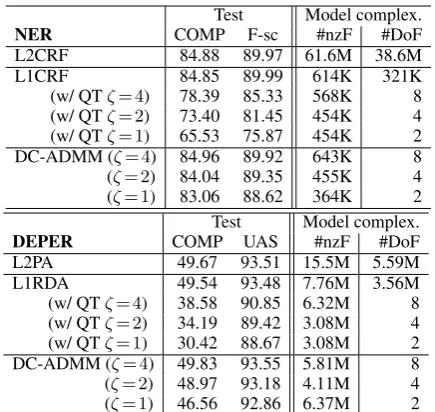
Fig. 3 shows the task performance on the develop-ment data against the model complexities in terms of the degrees of freedom in the trained models. Plots are given by changing theζ value for DC-ADMM andL1-regularized methods with QT. The plots of the standard L1-regularized methods are given by changing the regularization constantsλ1. Moreover, Table 1 shows the final results of our experiments on the test data. The tunable param-eters were fixed at values that provided the best performance on the development data.
According to the figure and table, the most re-markable point is that DC-ADMM successfully maintained the task performance even if #DoF (the degree of freedom) was 8, and the performance drop-offs were surprisingly limited even if #DoF was 2, which is the upper bound of feature group-ing. Moreover, it is worth noting that the DC-ADMM performance is sometimes improved. The reason may be that such low degrees of freedom prevent over-fitting to the training data. Surpris-ingly, the simple quantization method (QT) pro-vided fairly good results. However, we empha-size that the models produced by the QT approach offer no guarantee as to the optimal solution. In contrast, DC-ADMM can truly provide the opti-mal solution of Eq. 3 since the discrete constraint is also considered during the model learning.
In general, a trained model consists of two parts:
Test Model complex.
NER COMP F-sc #nzF #DoF
L2CRF 84.88 89.97 61.6M 38.6M
L1CRF 84.85 89.99 614K 321K
(w/ QTζ= 4) 78.39 85.33 568K 8 (w/ QTζ= 2) 73.40 81.45 454K 4 (w/ QTζ= 1) 65.53 75.87 454K 2 DC-ADMM (ζ= 4) 84.96 89.92 643K 8
(ζ= 2) 84.04 89.35 455K 4
(ζ= 1) 83.06 88.62 364K 2 Test Model complex.
DEPER COMP UAS #nzF #DoF
L2PA 49.67 93.51 15.5M 5.59M
L1RDA 49.54 93.48 7.76M 3.56M
(w/ QTζ= 4) 38.58 90.85 6.32M 8 (w/ QTζ= 2) 34.19 89.42 3.08M 4 (w/ QTζ= 1) 30.42 88.67 3.08M 2 DC-ADMM (ζ= 4) 49.83 93.55 5.81M 8 (ζ= 2) 48.97 93.18 4.11M 4
(ζ= 1) 46.56 92.86 6.37M 2
Table 1: Comparison results of the methods on test data (K: thousand, M: million)
feature weights and an indexed structure of fea-ture strings, which are used as the key for obtain-ing the correspondobtain-ing feature weight. This paper mainly discussed how to reduce the size of the for-mer part, and described its successful reduction. We note that it is also possible to reduce the lat-ter part especially if the feature string structure is TRIE. We omit the details here since it is not the main topic of this paper, but by merging feature strings that have the same feature weights, the size of entire trained models in our DEPAR case can be reduced to about 10 times smaller than those ob-tained by standardL1-regularization,i.e., to 12.2 MB from 124.5 MB.
5 Conclusion
[image:5.595.75.293.62.195.2]References
Galen Andrew and Jianfeng Gao. 2007. Scal-able Training of L1-regularized Log-linear Models. In Zoubin Ghahramani, editor, Proceedings of the 24th Annual International Conference on Machine Learning (ICML 2007), pages 33–40. Omnipress.
Amir Beck and Marc Teboulle. 2009. A Fast Iter-ative Shrinkage-thresholding Algorithm for Linear Inverse Problems. SIAM Journal on Imaging Sci-ences, 2(1):183–202.
Howard D. Bondell and Brian J. Reich. 2008. Simulta-neous Regression Shrinkage, Variable Selection and Clustering of Predictors with OSCAR. Biometrics, 64(1):115.
Stephen Boyd, Neal Parikh, Eric Chu, Borja Peleato, and Jonathan Eckstein. 2011. Distributed Opti-mization and Statistical Learning via the Alternat-ing Direction Method of Multipliers. Foundations and Trends in Machine Learning.
Xavier Carreras. 2007. Experiments with a Higher-Order Projective Dependency Parser. In Proceed-ings of the CoNLL Shared Task Session of EMNLP-CoNLL 2007, pages 957–961.
Koby Crammer, Ofer Dekel, Joseph Keshet, Shai Shalev-Shwartz, and Yoram Singer. 2006. On-line Passive-Aggressive Algorithms. Journal of Ma-chine Learning Research, 7:551–585.
John Duchi and Yoram Singer. 2009. Efficient On-line and Batch Learning Using Forward Backward Splitting. Journal of Machine Learning Research, 10:2899–2934.
Kevin Duh, Jun Suzuki, and Masaaki Nagata. 2011. Distributed Learning-to-Rank on Streaming Data using Alternating Direction Method of Multipliers. InNIPS’11 Big Learning Workshop.
Hugh Everett. 1963. Generalized Lagrange Multiplier Method for Solving Problems of Optimum Alloca-tion of Resources. Operations Research, 11(3):399– 417.
Daniel Gabay and Bertrand Mercier. 1976. A Dual Algorithm for the Solution of Nonlinear Variational Problems via Finite Element Approximation. Com-puters and Mathematics with Applications, 2(1):17 – 40.
Jianfeng Gao, Galen Andrew, Mark Johnson, and Kristina Toutanova. 2007. A comparative study of parameter estimation methods for statistical natural language processing. InProceedings of the 45th An-nual Meeting of the Association of Computational Linguistics, pages 824–831, Prague, Czech Repub-lic, June. Association for Computational Linguis-tics.
Rebecka J¨ornsten and Bin Yu. 2003. Simulta-neous Gene Clustering and Subset Selection for
Sample Classification Via MDL. Bioinformatics, 19(9):1100–1109.
Terry Koo, Xavier Carreras, and Michael Collins. 2008. Simple Semi-supervised Dependency Pars-ing. In Proceedings of ACL-08: HLT, pages 595– 603.
John Lafferty, Andrew McCallum, and Fernando Pereira. 2001. Conditional Random Fields: Prob-abilistic Models for Segmenting and Labeling Se-quence Data. In Proceedings of the International Conference on Machine Learning (ICML 2001), pages 282–289.
Dong C. Liu and Jorge Nocedal. 1989. On the Limited Memory BFGS Method for Large Scale Optimiza-tion. Math. Programming, Ser. B, 45(3):503–528.
Mitchell P. Marcus, Beatrice Santorini, and Mary Ann Marcinkiewicz. 1994. Building a Large Annotated Corpus of English: The Penn Treebank. Computa-tional Linguistics, 19(2):313–330.
Ryan McDonald, Koby Crammer, and Fernando Pereira. 2005. Online Large-margin Training of Dependency Parsers. InProceedings of the 43rd An-nual Meeting on Association for Computational Lin-guistics, pages 91–98.
Xiaotong Shen and Hsin-Cheng Huang. 2010. Group-ing Pursuit Through a Regularization Solution Sur-face. Journal of the American Statistical Associa-tion, 105(490):727–739.
Robert Tibshirani, Michael Saunders, Saharon Ros-set, Ji Zhu, and Keith Knight. 2005. Sparsity and Smoothness via the Fused Lasso. Journal of the Royal Statistical Society Series B, pages 91–108.
Erik Tjong Kim Sang and Fien De Meulder. 2003. Introduction to the CoNLL-2003 Shared Task: Language-Independent Named Entity Recognition. InProceedings of CoNLL-2003, pages 142–147. Yoshimasa Tsuruoka, Jun’ichi Tsujii, and Sophia
Ana-niadou. 2009. Stochastic Gradient Descent Training for L1-regularized Log-linear Models with Cumu-lative Penalty. InProceedings of the Joint Confer-ence of the 47th Annual Meeting of the ACL and the 4th International Joint Conference on Natural Lan-guage Processing of the AFNLP, pages 477–485.
Lin Xiao. 2010. Dual Averaging Methods for Regular-ized Stochastic Learning and Online Optimization.
Journal of Machine Learning Research, 11:2543– 2596.
Leon Wenliang Zhong and James T. Kwok. 2011. Efficient Sparse Modeling with Automatic Feature Grouping. InICML.