Munich Personal RePEc Archive
Bayesian Nonparametric Estimation of
Ex-post Variance
Griffin, Jim and Liu, Jia and Maheu, John M
University of Kent, McMaster University, McMaster University
10 May 2016
Online at
https://mpra.ub.uni-muenchen.de/71220/
Bayesian Nonparametric Estimation of Ex-post Variance
∗
Jim Griffin
†Jia Liu
‡John M. Maheu
§April, 2016
Abstract
Variance estimation is central to many questions in finance and economics. Until now ex-post variance estimation has been based on infill asymptotic assumptions that exploit high-frequency data. This paper offers a new exact finite sample approach to estimating ex-post variance using Bayesian nonparametric methods. In contrast to the classical counterpart, the proposed method exploits pooling over high-frequency obser-vations with similar variances. Bayesian nonparametric variance estimators under no noise, heteroskedastic and serially correlated microstructure noise are introduced and discussed. Monte Carlo simulation results show that the proposed approach can in-crease the accuracy of variance estimation. Applications to equity data and comparison with realized variance and realized kernel estimators are included.
∗We are grateful for comments from seminar participants at the 2016 NBER-NSF Seminar on Bayesian
Inference in Econometrics and Statistics. Maheu thanks the SSHRC of Canada for financial suport.
†School of Mathematics, Statistics and Actuarial Science, University of Kent, UK,
‡DeGroote School of Business, McMaster University, Canada, [email protected]
1
Introduction
This paper introduces a new method of estimating ex-post volatility from high-frequency data using a Bayesian nonparametric model. The proposed method allows the data to cluster under a flexible framework. In contrast to existing classical estimation methods, it delivers an exact finite sample distribution for the ex-post variance or transformations of the variance. Bayesian nonparametric variance estimators under no noise, heteroskedastic and serially correlated microstructure noise are proposed.
Volatility is an indispensable quantity in finance and is a key input into asset pricing, risk management and portfolio management. In the last two decades, researchers have taken advantage of high-frequency data to estimate ex-post variance using intraperiod returns. Barndorff-Nielsen & Shephard (2002) and Andersen et al. (2003) formalized the idea of using high frequency data to measure the volatility of lower frequency returns. They show that realized variance (RV) is a consistent estimator of quadratic variation under ideal conditions. Unlike parametric models of volatility in which the model specification is important, RV is a model free estimate of quadratic variation in that it is valid under a wide range of spot volatility dynamics.1
RV provides an accurate measure of ex-post variance if there is no market microstructure noise. However, observed prices at high-frequency are inevitably contaminated by noise in reality and returns are no longer uncorrelated. In this case, RV is a biased and inconsistent estimator (Hansen & Lunde 2006, A¨ıt-Sahalia et al. 2011). The impact of market microstruc-ture noise on forecasting is explored in A¨ıt-Sahalia & Mancini (2008) and Andersen et al. (2011).
Several different approaches have been proposed to estimating ex-post variance under microstructure noise. Zhou (1996) first introduced the idea of using a kernel-based method to estimate ex-post variance. Barndorff-Nielsen et al. (2008) formally discussed the real-ized kernel and showed how to use it in practice in a later paper (Barndorff-Nielsen et al. (2009)). Another approach is the subsampling method of Zhang et al. (2005). Hansen et al. (2008) showed how a time-series model can be used to filter out market microstructure to obtain corrected estimates of ex-post variance. A robust version of the predictive density of integrated volatility is derived in Corradi et al. (2009). Although bootstrap refinements are explored in Goncalves & Meddahi (2009) all distributional results from this literature rely on in-fill asymptotics.
Our Bayesian approach introduces a new concept to this problem, pooling. The existing ex-post variance estimators treat the information on variance from all intraperiod returns independently. However, the variance of intraperiod returns may be the same at different time periods. Pooling observations with common variance level may be beneficial to daily variance estimation.
We model intraperiod returns according to a Dirichlet process mixture (DPM) model. This is a countably infinite mixture of distributions which facilitates the clustering of return observations into distinct groups sharing the same variance parameter. The DPM model be-came popular for density estimation following the introduction of Markov chain Monte Carlo
1For a good survey of the key concepts see Andersen & Benzoni (2008), for an in-depth treatment see
(MCMC) techniques by Escobar & West (1994). Estimation of these models is now standard with several alternatives available, see Neal (2000) and Kalli et al. (2011). Our proposed method benefits variance estimation in at least three aspects. First, the common values of intraperiod variance can be pooled into the same group leading to a more precise estimate. The pooling is done endogenously along with estimation of other model parameters. Second, the Bayesian nonparametric model delivers exact finite inference regarding ex-post variance or transformations such as the logarithm. As such, uncertainty around the estimate of ex-post volatility is readily available from the predictive density. Unlike the existing asymptotic theory which may give confidence intervals that contain negative values for variance, density intervals are always on the positive real line and can accommodate asymmetry.
By extending key results in Hansen et al. (2008) we adapt the DPM mixture models to deal with returns contaminated with heteroskedastic noise and serially correlated noise.
Monte Carlo simulation results show the Bayesian approach to be a very competitive alternative. Overall, pooling can lead to more precise estimates of ex-post variance and better coverage frequencies. We show that the new variance estimators can be used with confidence and effectively recover both the average statistical features of daily ex-post variance as well as the time-series properties. Two applications to real world data with comparison to realized variance and kernel-based estimators are included.
This paper is organized as follows. In section 2, we provide a brief review of some existing variance estimators which serve as the benchmarks for later comparison. The Bayesian non-parametric model, daily variance estimator and model estimation methods are discussed in Section 3. Section 4 extends the Bayesian nonparametric model to deal with heteroskedastic and serially correlated microstructure noise. Section 5 provides an extensive simulation and comparison of the estimators. Applications to IBM and Disney data are found in Section 6. Section 7 concludes followed by an appendix.
2
Existing Ex-post Volatility Estimation
2.1
Realized Variance
Realized variance (RV), which equals the summation of squared intraperiod returns, is the most commonly used ex-post volatility measurement. Andersen et al. (2003) and Barndorff-Nielsen & Shephard (2002) formally studied the properties of RV and show it is a consistent estimator of quadratic variation under no microstructure noise. We will focus on variance estimation over a day t but all of the papers results apply to other time intervals.
Under the assumption of frictionless market and semimartingle, considering the following log-price diffusion,
dp(t) = µ(t) dt+σ(t) dW(t), (1)
where p(t) denotes the log-price at time t, µ(t) is the drift term, σ2(t) is the spot variance
and W(t) a standard Brownian motion. If the price process contains no jump, the variation of the return overt−1 to t is measured by IVt,
IVt= Z t
t−1
Let rt,i denotes theith intraday return on day t, i= 1, . . . , nt, wherent is the number of intraday returns on day t. Realized variance is defined as
RVt= nt
X
i=1
r2t,i, (3)
and RVt p
−
→IVt, as nt→ ∞ (Andersen, Bollerslev, Diebold & Labys 2001).
Barndorff-Nielsen & Shephard (2002) derive the asymptotic distribution of RVt as
√n
t 1
√
2IQt
(RVt−IVt) d
−
→N(0,1), as nt → ∞, (4)
whereIQtstands for the integrated quarticity, which can be estimated by realized quarticity (RQt) defined as
RQt=
nt 3
nt
X
i=1
r4t,i −→p IQt, as nt→ ∞. (5)
2.1.1 Flat-top Realized Kernel
If returns are contaminated with microstructure noise, RVt will be biased and inconsistent (Zhang et al. 2005, Hansen & Lunde 2006, Bandi & Russell 2008). The observed log-price ˜
pt,i, is assumed to follow
˜
pt,i =pt,i+ǫt,i, (6)
wherept,i is the true but latent log-price and ǫt,i is a noise term which is independent of the price.
Barndorff-Nielsen et al. (2008) introduced the flat-top realized kernel (RKF
t ), which is the optimal estimator if the microstructure error is a white noise process2.
RKtF = nt
X
i=1
˜
rt,i2 + H X
h=1
k
h−1
H
(γ−h+γh), γh = nt
X
i=1
˜
rt,i˜rt,i−h, (7)
where H is the bandwidth,k(x) is a kernel weight function.
The preferred kernel function is the second order Tukey-Hanning kernel3and the preferred bandwidth isH∗ =cξ√nt, whereξ2 =ω2/√IQ
tdenotes the noise-to-signal ratio. ω2 stands for the variance of microstructure noise and can be estimated by RVt/(2nt) by Bandi & Russell (2008). RVt based on 10-minute returns is less sensitive to microstructure noise and can be used as a proxy of √IQt. c= 5.74 given Tukey-Hanning kernel of order 2.
Given the Tukey-Hanning kernel and H∗ = cξ√nt, Barndorff-Nielsen et al. (2008) show
that the asymptotic distribution of RKtF is
n1t/4 RKtF −IVt
d
−
→MN
0,4IQ3t/4ω
ck0•,0+ 2c−1k•1,1√IVt
IQt
+c−3k•2,2
, (8)
2Another popular approach to dealing with noise is subsampling. See Zhang et al. (2005), A¨ıt-Sahalia &
Mancini (2008) for the Two Scales Realized Volatility (TSRV) estimator.
3Tukey-Hanning kernel with order 2: k(x) = sin2π
2(1−x)2
where MN is mixture of normal distribution, k0,0
• = 0.219, k•1,1 = 1.71 and k•2,2 = 41.7 for
second order Tukey-Hanning kernel.
Even though ω2 can be estimated using RV
t/(2nt), a better and less biased estimator suggested by Barndorff-Nielsen et al. (2008) is
ˇ
ω2 = explog(ˆω2)−RKt/RVt
. (9)
The estimation of IQt is more sensitive to the microstructure noise. The tri-power quar-ticity (T P Qt) developed by Barndorff-Nielsen & Shephard (2006) can be used to estimate
IQt,
T P Qt =ntµ−34/3 nXt−2
i=1
|r˜t,i|4/3|r˜t,i+1|4/3|r˜t,i+2|4/3, (10)
where µ4/3 = 22/3Γ(7/6)/Γ(1/2). Replacing IVt, ω2 and IQt with RKtF, ˇω2 and T P Qt in equation (8), the asymptotic variance of RKF
t can be calculated.
2.1.2 Non-negative Realized Kernel
The flat-top realized kernel discussed in previous subsection is based on the assumption that error term is white noise. However, the white noise assumption is restrictive and error term can be serial dependent or dependent with returns in reality. Another drawback of theRKF
t is that it may provide negative volatility estimates, all be it very rarely. Barndorff-Nielsen et al. (2011) further introduced the non-negative realized kernel (RKtN) which is more robust to these assumptions of error term and is calculated as
RKtN = H X
h=−H
k
h H+ 1
γh, γh = nt
X
i=|h|+1
˜
rt,ir˜t,i−|h|. (11)
The optimal choice of H is H∗ = cξ4/5n3/5
t and the preferred kernel weight function is the Parzen kernel4, which implies c = 3.5134. ξ2 can be estimated using the same method
as in the calculation of RKF t .
Barndorff-Nielsen et al. (2011) show the asymptotic distribution of RKN
t based onH∗ =
cξ4/5n3/5
t is given by
n1t/5 RKtN −IVt
d
−
→MN(κ,4κ2), (12)
where κ = κ0(IQtω)2/5, κ0 = 0.97 for Parzen kernel function, ω and IQt can be estimated using equation (9) and (10).
Note that RKN
t is no longer a consistent estimator of IVt and the rate of convergence is slower than that of RKF
t . If the error term is white noise, RKtF is superior to RKtN, but
RKN
t is more robust to deviations from independent noise and is always positive.
4Parzen kernel function:
k(x) =
1−6x2+ 6x3, 0≤x≤1/2
2(1−x)3, 1/2< x≤1
3
Bayesian Nonparametric Ex-post Variance
Estima-tion
In this section, we introduce a Bayesian nonparametric ex-post volatility estimator. After defining the daily variance, conditional on the data, the discussion moves to the DPM model which provides the model framework of the proposed estimator. The approach discussed in this section deals with returns without microstructure noise and an estimator suitable for returns with microstructure noise is found in Section 4.
3.1
Model of High-frequency Returns
First we consider the case with no market microstructure noise. The model for log-returns is
rt,i =µt+σt,izt,i, zt,i iid
∼ N(0,1), i= 1, . . . , nt, (13)
where µt is constant in day t. The daily return is
rt= nt
X
i=1
rt,i (14)
and it follows, conditional on the unknown realized volatility pathFt≡ {σt,i2 }ni=1t , the ex-post
variance is
Vt≡Var(rt|Ft) = nt
X
i=1
σ2t,i. (15)
In our Bayesian setting Vt is the target to estimate conditional on the data {rt,i}ni=1t . Note,
that we make no assumptions on the stochastic process generating σ2
t,i.
3.2
A Bayesian Model with Pooling
In this section we discuss a nonparametric prior for the model of (13) that allows for pooling over common values of σ2
t,i. The Dirichlet process mixture model (DPM) is a Bayesian nonparametric mixture model that has been used in density estimation and for modeling unknown hierarchical effects among many other applications. A key advantage of the model is that it naturally incorporates parameter pooling.
Our nonparametric model has the following hierarchical form
rt,i µt, σt,i
iid
∼ N(µt, σ2t,i), i= 1, . . . , nt, (16)
σt,i2 Gt iid
∼ Gt, (17)
Gt
G0,t, αt ∼ DP(αt, G0,t), (18)
G0,t(σ2t,i) ≡ IG(v0,t, s0,t), (19)
The Dirichlet process was formally introduced by Ferguson (1973) and is a distribution over distributions. A draw from a DP(αt, G0,t) is an almost surely discrete distribution which
is centered around the base distribution G0,t. Therefore, a sample from σt,i2
Gt ∼ Gt has a positive probability of repeated values. The concentration parameter αt > 0 governs how closely a draw Gt resembles G0,t. Larger values of αt lead to Gt having the more unique atoms with significant weights. As αt → ∞, Gt → G0,t which implies that every rt,i has a unique σ2
t,i drawn from the inverse-gamma distribution. In this case there is no pooling and we have a setting very close to the classical counterpart discussed above. However, for finite
αt, pooling can take place. The other extreme is complete pooling forαt→0 in which there is one common variance shared by all observations such thatσt,i2 =σt,21,∀i. Since αtplays an important role in pooling we place a prior on it and estimate it along with the other model parameters for each day.
A stick breaking representation (Sethuraman (1994)) of the DPM in (17) is given as follows.
p(rt,i
µt,Ψt, wt) =
∞
X
j=1
wt,jN(rt,i|µt, ψ2t,j), (20)
wt,j = vt,j j−1
Y
l=1
(1−wt,l), (21)
vt,j iid
∼ Beta(1, αt), (22)
where N(·|·,·) denotes the density of the normal distribution, Ψt={ψ2
t,1, ψ2t,2. . . . ,}is the set
of unique values of σ2
t,i, wt ={wt,1, wt,2, . . . ,} and wt,j is the weight associated with the jth component. This formulation of the model facilitates posterior sampling which is discussed in the next section.
Since our focus is on intraday returns and the number of observations in a day can be small, especially for lower frequencies such as 5-minute. Therefore, the prior should be chosen carefully. It is straightforward to show that the prior predictive distribution of σ2
t,i is G0,t.
Forσ2
t,i ∼IG(v0,t, s0,t), the mean and variance ofσt,i2 are
E(σt,i2 ) = s0,t
v0,t−1
and var(σ2t,i) = s
2 0,t
(v0,t−1)2(v0,t−2)
. (23)
Solving the two equations, the values ofv0,t and s0,t are given by
v0,t =
E(σ2
t,i) 2
var(σ2
t,i)
+ 2 and s0,t = E(σt,i2 )(v0,t−1). (24)
We use sample statistics var(c rt,i) and var(c r2
t,i) calculated with three days intraday returns (dayt−1, dayt, and dayt+1) to set the values of E(σ2
t,i) and var(σ2t,i), then use equation (24) to findv0,tands0,t. A shrinkage prior N(0, v2) is used forµtsinceµtis expected to be close to zero. v2 is small and adjusted according to the data frequency. Finally, α
t ∼Gamma(a, b). For a finite dataset i= 1, . . . , nt our target is the following posterior moment
E[Vt|{rt,i}ni=1t ] =E
" n
t
X
i=1
σt,i2
{rt,i}ni=1t
#
Note that the posterior mean of Vt can also be considered as the posterior mean of realized variance,RVt=Pni=1t rt,i2 assuming µt is small. As such,RVt treats eachσt,i2 as separate and corresponds to no pooling. We discuss estimation of the model next.
3.3
Model Estimation
Estimation relies on Markov chain Monte Carlo (MCMC) techniques. We apply the slice sampler of Kalli et al. (2011), along with Gibbs sampling to estimate the DPM model. The slice sampler provides an elegant way to deal with the infinite states in (20). It introduces an auxiliary variable ut,1:nt = {ut,1, . . . , ut,nt} that randomly truncates the state space to a
finite set at each MCMC iteration but marginally delivers draws from the desired posterior. The joint distribution of rt,i and the auxiliary variableut,i is given by
f(rt,i, ut,i|wt, µt,Ψt) =
∞
X
j=1
1(ut,i < wt,j) N rt,i|µt, ψ2t,j
, (26)
and integrating out ut,i recovers (20).
It is convenient to rewrite the model in terms of a latent state variable st,i ∈ {1,2, . . .} that maps each observation to an associated component and parameter σ2t,i = ψt,s2 t,i.
Ob-servations with a common state share the same variance parameter. For finite dataset the number of states (clusters) is finite and ordered from 1, . . . , K. Note that the number of clusters K, is not a fixed value over the MCMC iterations. A new cluster with variance
ψ2
t,K+1 ∼G0,t can be created if existing clusters do not fit that observation well and clusters sharing a similar variance can be merged into one.
The joint posterior is
p(µt) K Y
j=1
p(ψ2
t,j)
p(αt) nt
Y
i=1
1(ut,i < wt,st,i)N(rt,i|µt, ψ 2
t,st,i). (27)
Each MCMC iteration contains the following sampling steps.
1. π µt|rt,1:nt,{ψ 2
t,j}Kj=1, st,1:nt
∝p(µt)Qnt
i=1p
rt,i
µt, ψ2t,st,i
.
2. π ψ2
t,j|rt,1:nt, st,1:nt, µt
∝p ψ2
t,j Q
t:st,i=jp rt,i µt, ψt,j2
for j = 1, . . . , K.
3. π(vt,j|st,1:nt) ∝ Beta (vt,j|at,j, bt,j) with at,j = 1 +
Pnt
i=11(st,i =j) and bt,j = αt +
Pnt
i=11(st,i > j) and update wt,j =vt,j
Q
l<j(1−vt,l) for j = 1, . . . , K.
4. π(ut,i|wt,i, st,1:nt)∝1 0< ut,i < wt,st,i
.
5. Find the smallest K such that PKj=1wt,j >1−min (ut,1:nt).
6. π st,i|r1:nt, st,1:nt, µt,{ψ 2
t,j}Kj=1, ut,1:nt, K
∝ PKj=11(ut,i < wt,j)p rt,i,|µt, ψt,j2
for i = 1, . . . , nt.
In the first step µt is common to all returns and this is a standard Gibbs step given the conjugate prior. Step 2 is a standard Gibbs step for each variance parameter ψ2
t,j based on the data assigned to cluster j. The remaining steps are standard for slice sampling of DPM models. In 7,αt is sampled based on Escobar & West (1994).
Steps 1-7 give one iteration of the posterior sampler. After dropping a suitable burn-in amount,M additional samples are collected,{θ(m)}M
m=1, whereθ ={µt, ψt,21, . . . , ψt,K2 , st,1:nt, αt}.
Posterior moments of interest can be estimated from sample averages of the MCMC output.
3.4
Ex-post Variance Estimator
Conditional on the parameter vector θ the estimate of Vt is
E[Vt|θ] = nt
X
i=1
σ2t,si. (28)
The posterior mean of Vt is obtained by integrating out all parameter and distributional uncertainty. E[Vt|{rt,i}ni=1t ] is estimated as
ˆ
Vt = 1
M
M X
m=1
nt
X
i=1
σt,i2(m), (29)
where σt,i2(m) =ψ2(m)
t,s(m)t,i . Similarly other features of the posterior distribution of Vt can be ob-tained. For instance, a (1-α) probability density interval forVt is the quantiles ofPni=1t σ2t,st,i
associated with probabilities α/2 and (1−α/2). Conditional on the model and prior these are exact finite sample estimates, in contrast to the classical estimator which relies on infill asymptotics to derived confidence intervals.
If log(Vt) is the quantity of interest, the estimator of E[log(Vt)|{rt,i}ni=1t ] is given as
\
log(Vt) = 1
M
M X
m=1
log nt
X
i=1
σ2(t,im)
!
. (30)
As before, quantile estimates of the posterior of log(Vt) can be estimated from the MCMC output.
4
Bayesian Estimator Under Microstructure Error
4.1
DPM-MA(1) Model
The existence of microstructure noise turns the intraday return process into an autocorrelated process. First consider the case in which the error is white noise:
˜
pt,i =pt,i+ǫt,i, ǫt,i ∼N(0, ω2t,i), (31)
where ˜pt,i denotes the observed log-price with error,pt,i is the unobserved fundamental log-price and ω2
t,i is the heteroskedastic noise variance.
Given this structure it can be shown that the returns series ˜rt,i = ˜pt+1,i−p˜t,i has non-zero first order autocorrelation but zero higher order autocorrelation. That is cov(˜rt,i+1,˜rt,i) =
−ω2
t,i and cov(˜rt,i+j,r˜t,i) = 0 for j ≥2. This suggest a moving average model of order one. Combining MA(1) parameterization with our Bayesian nonparametric framework yields the DPM-MA(1) models.
˜
rt,i|µt, θt, δt,i2 = µt+θtηt,i−1+ηt,i, ηt,i ∼N(0, δt,i2 ) (32)
δ2t,i|Gt ∼ Gt, (33)
Gt|G0,t, αt ∼ DP(αt, G0,t), (34)
G0,t(δt,i2 ) ≡ IG(v0,t, s0,t). (35)
The noise terms are heteroskedastic. Note that the mean of rt,i is not a constant term but a moving average term. The MA parameter θt is constant for i but will change with the day t. The prior is θt ∼ N(mθ, vθ2)1{|θt|<1} in order to make the MA model invertible. The
error term ηt,0 is assumed to be zero. Other model settings remain the same as the DPM
illustrated in Section 3. Later we show how estimates from this specification can be be used to recover an estimate of the ex-post variance Vt of the true return process.
4.2
DPM-MA(q) Model
For lower sampling frequencies, such as 1 minute or more, first order autocorrelation is the main effect from market microstructure. As such, the MA(1) model will be sufficient for many applications. However, at higher sampling frequencies, the dependence may be stronger. To allow for a more complex effect on returns from the noise process consider the MA(q-1) noise affecting returns,
˜
pt,i =pt,i+ǫt,i−ρ1ǫt,i−1− · · · −ρq−1ǫt,i−q+1, ǫt,i ∼N(0, ω2t,i). (36)
For returns, this leads to the following DPM-MA(q) model,
˜
rt,i|µt,{θt,j}qj=1, δt,i2 = µt+ q X
j=1
θt,jηt,i−j +ηt,i, ηt,i ∼N(0, δt,i2 ) (37)
δt,i2 |Gt ∼ Gt, (38)
Gt|G0,t, αt ∼ DP(αt, G0,t), (39)
G0,t(δt,i2 ) ≡ IG(v0,t, s0,t). (40)
The joint prior of (θt,1, . . . , θt,q) is N(MΘ, VΘ)1{Θ}5 and (ηt,0, . . . , ηt,−(q−1)) = (0, . . . ,0).
5Restrictions on MA coefficients: all the roots of 1 +θ1B+θ2B2+· · ·+θ
qBq= 0 are outside of the unit
4.3
Model Estimation
We discuss the estimation of DPM-MA(1) model and the approach can be easily extended to the DPM-MA(q). The main difference in this model is that the conditional mean parameters
µtandθtrequire a Metropolis-Hasting (MH) step to sample their conditional posteriors. The remaining MCMC steps are essentially the same. As before, letψ2
t,i denote the unique values of δ2
t,j then each MCMC iteration samples from the following conditional distributions.
1. π µt|˜rt,1:nt,{ψ 2
t,j}Kj=1, θt, st,1:nt
∝p(µt)Qnt
i=1N
˜
rt,i|µt+θtηt,i−1, ψ2t,st,i
.
2. π θt|r˜t,1:nt, µt,{ψ 2
t,j}Kj=1, st1:nt
∝p(θt)Qnt
i=1p
˜
rt,i|µt+θtηt,i−1, ψt,s2 t,i
.
3. π ψ2
t,j|r˜t,1:nt, µt, θt, st,1:nt
∝p ψ2
t,j Q
t:st=jp r˜t,i|µt+θtεt,i−1, ψ2t,j
forj = 1, . . . , K.
4. π(vt,j|st,1:nt) ∝ Beta (vt,j|at,j, bt,j) with at,j = 1 +
Pnt
i=11(st,i = j) and bt,j = αt+
Pnt
i=11(st,i > j) and update wt,j =vt,jQl<j(1−vt,l) for j = 1, . . . , K.
5. π(ut,i|wt,i, st,1:nt)∝1(0< ut,i < wt,st,i) for i= 1, . . . , nt.
6. Find the smallest K such that PKj=1wt,j >1−min(ut,1:nt).
7. π st,i|r˜1:nt, st,1:nt, µt, θt,{ψ 2
t,j}Kj=1, ut,1:nt, K
∝PKj=11(ut,i < wt,j)N(˜rt,i|µt+θtηt,i−1, ψt,j2 ) for i= 1, . . . , nt.
8. π(αt|K)∝p(αt)p(K|αt).
In steps 1 and 2 the likelihood requires the sequential calculation of the lagged error as
ηt,i−1 = ˜rt,i−1−µt−θtηt,i−2 which precludes a Gibbs sampling step. Therefore, µt and θt are sampled using a MH with a random walk proposal. The proposal is calibrated to achieve an acceptance rate between 0.3 and 0.5.
4.4
Ex-post Variance Estimator under Microstructure Error
Hansen et al. (2008) showed that prefiltering with an MA model results in a bias in the RV estimator.6 In the Appendix it is shown that the Hansen et al. (2008) bias correction provides
an accurate adjustment to our Bayesian estimator in the context of heteroskedastic noise. From the DPM-MA(1) model the posterior mean of Vt under independent microstructure error is
ˆ
Vt,MA(1) =
1
M
M X
m=1
(1 +θt(m))2 nt
X
i=1
δt,i2(m), (41)
where δt,i2(m)=ψ2(m)
t,s(m)t,i The log of Vt, square-root ofVt and density intervals can be estimated as the Bayesian nonparametric ex-post variance estimator without microstructure error.
6If ˜r
t=θ1ηt−1+· · ·+θqηt−q+1+ηt, then under their assumptions the bias corrected estimate of ex-post
variance isRVMAq= (1 +θ1+· · ·+θq)2 nt P
i=1
ˆ
η2
In the case of higher autocorrelation the DPM-MA(q) model adjusted posterior estimate of Vt is
ˆ
Vt,MA(q)=
1
M
M X
m=1
1 + q X
j=1
θt,j(m)
!2 nt
X
i=1
δ2(t,im). (42)
Next we consider simulation evidence on these estimators.
5
Simulation Results
5.1
Data Generating Process
We consider four commonly used data generating processes (DGPs) in the literature. The first one is the GARCH(1,1) diffusion, introduced by Andersen & Bollerslev (1998). The log-price follows
dp(t) =µdt+σ(t)dWp(t), (43) dσ2(t) =α(β−σ2(t))dt+γσ2(t)dWσ(t). (44)
where Wp(t) and Wσ(t) are two independent Wiener processes. The values of parameters follow Andersen & Bollerslev (1998) and areµ= 0.03, α= 0.035, β = 0.636 and γ = 0.144, which were estimated using foreign exchange data.
Following Huang & Tauchen (2005), the second and third DGP are a one factor stochastic volatility diffusion (SV1F) and one factor stochastic volatility diffusion with jumps (SV1FJ). SV1F is given by
dp(t) =µdt+ exp (β0+β1v(t)) dWp(t), (45)
dv(t) = αv(t)dt+ dWv(t) (46)
and the process for SV1FJ is
dp(t) = µdt+ exp (β0 +β1v(t)) dWp(t) +dJ(t) , (47) dv(t) = αv(t)dt+ dWv(t), (48)
where corr(dWp(t),dWv(t)) = ρ, and J(t) is a Poisson process with jump intensity λ and jump size δ ∼ N(0, σ2
J). We adopt the parameter settings from Huang & Tauchen (2005) and set µ= 0.03, β0 = 0.0,β1 = 0.125, α=−0.1, ρ=−0.62, λ = 0.014 and σJ2 = 0.5.
The final DGP is the two factor stochastic volatility diffusion (SV2F) from Chernov et al. (2003) and Huang & Tauchen (2005).7
dp(t) = µdt+s- exp (β0+β1v1(t) +β2v2(t)) dWp(t), (49) dv1(t) =α1v1(t)dt+ dWv1(t), (50)
dv2(t) =α2v2(t)dt+ (1 +ψv2(t)) dWv2(t), (51)
7The functions- exp is defined ass- exp(x) = exp(x) if x≤x0 and s- exp(x) = exp(x0)
√x
0 p
x0−x2
0+x2 if
where corr(dWp(t),dWv1(t)) =ρ1 and corr(dWp(t),dWv2(t)) =ρ2. The parameter values in
SV2F are µ= 0.03, β0 =−1.2, β1 = 0.04, β2 = 1.5, α1 =−0.00137, α2 =−1.386, ψ = 0.25
and ρ1 =ρ2 =−0.3, which are from Huang & Tauchen (2005).
Data is simulated using a basic Euler discretization at 1-second frequency for the four DGPs. Assuming the length of daily trading time is 6.5 hours (23400 seconds), we first simulate the log price level every second. After this we compute the 5-minute, 1-minute, 30-second and 10-second intraday returns by taking the difference every 300, 60, 30, 10 steps, respectively. The initial volatility level, such as v1t and v2t in SV2F, at day t is set equal to the last volatility value at previous day, t−1. T = 5000 days of intraday returns are simulated using the four DGPs and used to report sampling properties of the volatility estimators. In each case, to remove dependence on the startup conditions 500 initial days are dropped from the simulation.
5.1.1 Independent Noise
Following Barndorff-Nielsen et al. (2008), log-prices with independent noise are simulated as follows
˜
pt,i =pt,i−1 +ǫt,i,
ǫt,i ∼N(0, σω2),
σ2ω =ξ2var(rt).
(52)
The error term is added to the log-prices simulated from the 4 DGPs every second. The variance of microstructure error is proportional to the daily variance calculated using the pure daily returns. We set the noise-to-signal ratio ξ2 = 0.001, which is the same value used
in Barndorff-Nielsen et al. (2008) and close to the value in Bandi & Russell (2008).
5.1.2 Dependent Noise
Following Hansen et al. (2008), we consider the simulation of log-prices with dependent noise as follows,
˜
pt,i =pt,i−1+ǫt,i,
ǫt,i ∼N µǫt,i, σ 2
ω
,
µǫt,i =
φ X
l=1
(1−l/φ) (pt,i−l−pt,i−1−l),
σ2ω =ξ2var(rt),
(53)
where φ = 20, which makes the error term correlated with returns in the past 20 seconds (steps). If past returns are positive (negative) the noise term tends to be positive (negative). All other settings, such as σ2
ω and ξ2, are the same as in the independent error case.
5.2
True Volatility and Comparison Criteria
of the squared intraday pure returns at the highest frequency (1 second)
σ2t ≡
23400X
i=1
rt,i2 . (54)
The competing ex-post daily variance estimators, generically labeled ˆσ2
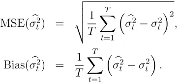
t, are compared based on the root mean squared errors (RMSE), and bias defined as
RMSE(σb2
t) =
v u u t1 T T X t=1 b σ2
t −σ2t 2
, (55)
Bias(σb2
t) =
1 T T X t=1 b σ2
t −σt2
. (56)
The coverage probability estimates report the frequency that the confidence intervals or density intervals from the Bayesian nonparametric estimators contain the true ex-post variance,σ2
t. The 95% confidence intervals of RVt, RKtF and RKtN reply on the asymptotic distribution, which are provided in equation (4), (8) and (12). We take the bias into account to compute the 95% confidence interval using RKN
t .
The estimation of integrated quarticity is crucial in determining the confidence interval for the realized kernels. We consider two versions of quarticity, one is to use the true (infeasible)
IQt which is calculated as
IQtruet = 23400
23400X
i=1
σ4t,i, (57)
where σ2
t,i refers to spot variance simulated at the highest frequency. The other method is to estimate IQt using the tri-power quarticity estimator, see formula (10). The confidence interval based on IQtrue
t is the infeasible case and the confidence interval calculated using
T P Qt is the feasible case.
For each day 5000 MCMC draws are collected after 1000 burn-in to compute the Bayesian posterior quantities. A 0.95 density interval is the 0.025 and 0.975 sample quantiles of MCMC draws of Pnt
i=1σ2t,i, respectively.
[image:15.612.219.399.188.274.2]5.3
No Microstructure Noise
Figure 1 plots 500 days of σ2
t and estimates RVt and ˆVt based on returns simulated from the GARCH(1,1) DGP at 5-minute, 1-minute, 30-second and 10-second. Both estimators become more accurate as the data frequency increases.
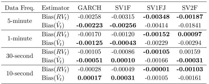
Table 3 shows the bias to be small for both estimators. The Bayesian estimator reduces the bias for data simulated from GARCH and SV1F diffusion, while RVthas smaller bias in the other cases.
Table 4 shows that coverage probabilities for 95% confidence intervals of RVt and 0.95 density intervals of ˆVt. The Bayesian nonparametric estimator produces fairly good coverage probabilities for both low and high frequency data, except for the SV2F data. For RVt, data frequencies higher than 5-minutes are needed to obtain good finite sample coverage when the asymptotic distribution is used.
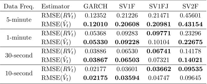
In summary, under no microstructure noise, the Bayesian nonparametric estimator is very competitive with the classical counterpart RVt. ˆVt offers smaller estimation error and better finite sample results than RVt when the data frequency is low. Performance of RVt and ˆVt both improve as the sampling frequency increases.
5.4
Independent Microstructure Noise
In this section we compare RVt, RKF
t , ˆVt and ˆVt,MA(1). Figure 3 displays the time-series of
RKF
t , ˆVt,MA(1) along with the true variance for several sampling frequencies for data from
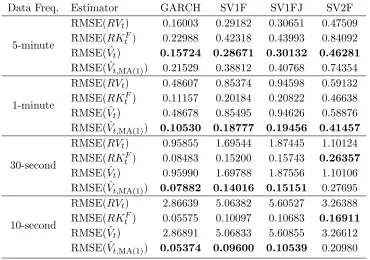
the SV1F DGP. Both estimators become more accurate as the sampling frequency increases. Table 5 shows the RMSE of the various estimators for different sampling frequencies and DGPs. RVt and ˆVt produce smaller errors in estimating σt2 than RKtF and ˆVt,MA(1) for
5-minute data. However, increasing the sampling frequency results in a larger bias from the microstructure noise. As such, RKF
t and ˆVt,MA(1) are more accurate as the data frequency
increases. Compared toRKF
t , ˆVt,MA(1) has a smaller RMSE in all cases, except for 30-second
and 10-second SV2F return. Figure 4 shows that ˆVt,MA(1) outperforms RKtF in most of the subsamples.
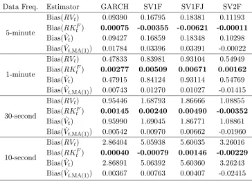
The bias of the estimators is found in Table 6. Again, RVt and ˆVt overestimate the ex-post variance by a significant amount unless the data frequency is low. Both RKF
t and
ˆ
Vt,MA(1) produce better results as more data is used. The bias ofRKtF is smaller than that
of ˆVt,MA(1), but the differences are minor.
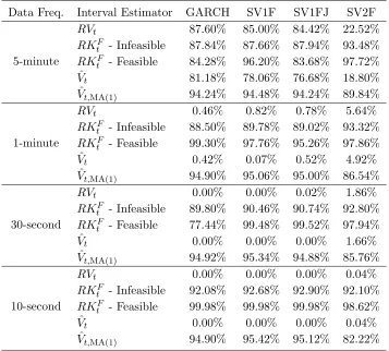
As can be seen in Table 7, ˆVt,MA(1) has the best finite sample coverage among all the
alternatives except for the SV2F data. For example, the coverage probabilities of 0.95 density intervals are always within 0.5% from the truth. Note that the density intervals are trivial to obtain from the MCMC output and do not require the calculation IQt. The coverage probabilities of either infeasible and feasible confidence intervals of realized kernels are not as good as those of ˆVt,MA(1). Moreover, RKtF requires larger samples for good coverage, while density intervals of ˆVt,MA(1) perform well for either low or high frequency returns.
5.5
Dependent Microstructure Noise
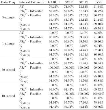
The last experiment considers the performances of the estimators under dependent noise.
RKN
t ,RVt, ˆVt, ˆVt,MA(1) and ˆVt,MA(2) are compared. Figure 5 plots the estimators for different
sampling frequencies. It is clear that estimation is less precise in this setting.
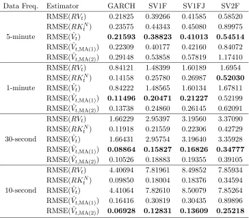
estimator has the smallest RMSE in each case. The ˆVt,MA(1) estimator is ranked the best
if return frequency is 30 seconds, followed by ˆVt,MA(2) and RKtN. For 10 seconds returns, ˆ
VMA(2) provides the smallest error. Compared to RKtN the ˆVt,MA(1) and ˆVt,MA(2) can provide
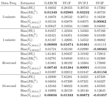
significant improvements for 30 and 10 second returns. For instance, at 30 seconds, reductions in the RMSE of 10% or more are common while at the 10 second frequency reductions in the RMSE are 25% or more. The subsample analysis shown in Figure 6 supports these findings. Table 9 shows ˆVt,MA(1) and ˆVt,MA(2) have smaller bias if return frequency is one minute or
higher.
Table 10 shows the coverage probabilities of all the five estimators. The finite sample results of ˆVt,MA(2) are all very close to the optimal level, no matter the data frequency.
5.6
Evidence of Pooling
Figure 7-9 display the histograms of the posterior mean of the number of clusters in three different settings. There are: the DPM for 5-minute SV1F returns (no noise), the DPM-MA(1) for 1-minute SV1FJ returns (independent noise) and the DPM-MA(2) for 30-second SV2F returns (dependent noise). The figures show significant pooling. For example, in the 1-minute SV1FJ return case, most of the daily variance estimates ofVt are formed by using 1 to 5 pooled groups of data, instead of 390 observations (separate groups) which is what the realized kernel uses. This level of pooling can lead to significant improvements for the Bayesian estimator.
In summary, these simulations show the Bayesian estimate of ex-post variance to be very competitive with existing classical alternatives.
6
Empirical Applications
For each day, 5000 MCMC draws are taken after 10000 burn-in draws are discarded, to estimate posterior moments. All prior setting are the same as in the simulations.
6.1
Application to IBM Return
We first consider estimating and forecasting volatility using a long calendar span of IBM equity returns. The 1-minute IBM price records from 1998/01/03 to 2016/02/16 were down-loaded from Kibot website8. We choose the sample starting from 2001/01/03 as the relatively small number of transactions before year 2000 yields many zero intraday returns. The days with less than 5 hours of trading are removed, which leaves 3764 days in the sample.
Log-prices are placed on a 1-minute grid using the price associated with closest time stamp that is less than or equal to the grid time. The 5-minute and 1-minute percentage log returns from 9:30 to 16:00(EST) are constructed by taking the log price difference between two close prices in time grid and scaling by 100. The overnight returns are ignored so the first intraday return is formed using the daily opening price instead of the close price in previous day. The procedure generates 293,520 5-minute returns and 1,467,848 1-minute returns.
We use a filter to remove errors and outliers caused by abnormal price records. We would like to filter out the situation in which the price jumps up or down but quickly moves back to original price range. This suggest an error in the record. If |rt,i|+|rt,i+1| >8
p
vart(rt,i) and |rt,i+rt,i+1|<0.05%, we replace rt,i and rt,i+1 by r′t,i =rt,i′ +1 = 0.5×(rt,i+rt,i+1). The
filter adjusts 0 and 70 (70/1,467,848 = 0.00477%) returns for 5-minute and 1-minute case, respectively.
From these data several version of daily ˆVt, RVt and RKt are computed. Daily returns are the open-to-close return and match the time interval for the variance estimates. For each of the estimators we follow exactly the methods used in the simulation section.
6.1.1 Ex-post Variance Estimation
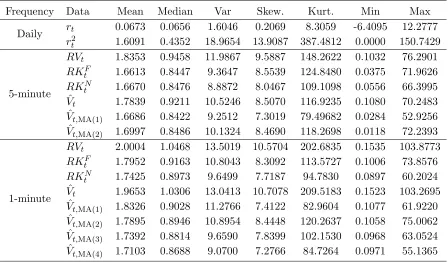
Table 11 reports summary statistics for several estimators. Overall the Bayesian and classical estimators are very close. Both the realized kernel and the moving average DPM estimators reduce the average level of daily variance and indicate the presence of significant market microstructure noise. Based on this and an analysis of the ACF of the high-frequency returns we suggest the ˆVt,MA(1) for the 5-minute data and the ˆVt,MA(4) for the 1-minute data in the
remainder of the analysis. Comparison with the kernel estimators is found in Figures 10 and 11. Except for the extreme values they are very similar.
Interval estimates for two sub-periods are shown in Figures 12 and 13. A clear disadvan-tage of the kernel based confidence interval in that it includes negative values for ex-post variance. The Bayesian version by construction does not and tends to be significantly shorter in volatile days. The results of log variance9 are also provided with some differences
remain-ing.
The degree of pooling from the Bayesian estimators is found in Figure 14 and 15. As expected, we see more groups in the higher 1-minute frequency. In this case, on average, there are about 3 to 7 distinct groups of intraday variance parameters.
6.1.2 Ex-post Variance Modeling and Forecasting
Does the Bayesian estimator correctly recover the time-series dynamics of volatility? To investigate this we estimate several versions of the Heterogeneous Auto-Regressive (HAR) model introduced by Corsi (2009). This is a popular model that captures the strong depen-dence in ex-post daily variance. For ˆVt the HAR model is
ˆ
Vt =β0+β1Vˆt−1+β2Vˆt−1|t−5+β3Vˆt−1|t−22+ǫt, (58)
where ˆVt−1|t−h = h1 Phl=1Vˆt−l andǫtis the error term. ˆVt−1, ˆVt−1|t−5 and ˆVt−1|t−22correspond
to the daily, weekly and monthly variance measures up to time t−1. Similar specifications are obtained by replacing ˆVt with RVt or RKt.
Bollerslev et al. (2016) extend the HAR model to the HARQ model by taking the asymp-totic theory of RVt into account. The HARQ model for RVt is given by
RVt =β0+
β1+β1QRQ1t−1/2
RVt−1+β2RVt−1|t−5+β3RVt−1|t−22+ǫt (59)
995% confidence intervals using log(RV
t), log(RKtF) and log(RKtN) are based on the asymptotic
The loading onRVt−1 is no longer a constant, but varying with measurement error, which is
captured byRQt−1. The model responds more to RVt−1 if measurement error is low and has
a lower response if error is high. Bollerslev et al. (2016) provide evidence that the HARQ model outperforms HAR model in forecasting.10
An advantage of our Bayesian approach is that we have the full finite sample posterior distribution for Vt. In the Bayesian nonparametric framework, there is no need to estimate
IQt with RQt, instead the variance, standard deviation or other features of Vt can be easily estimated using the MCMC output. Replacing RQt−1 with var(c Vt−1), the modified HARQ
model for ˆVt is defined as ˆ
Vt=β0+ β1+β1Qvar(c Vt−1)1/2
ˆ
Vt−1+β2Vˆt−1|t−5+β3Vˆt−1|t−22+ǫt, (60)
where var(c Vt−1)1/2 is an MCMC estimate of the posterior standard deviation ofVt.
Table 12 displays the OLS estimates and the R2 for several model specifications.
Coef-ficient estimates are comparable across each class of model. Clearly the Bayesian variance estimates display the same type of time-series dynamics found in the realized kernel esti-mates.
Finally, out-of-sample root-mean squared forecast errors (RMSFE) of HAR and HARQ models using both classical estimators and Bayesian estimators are found in Table 13. The out-of-sample period is from 2005/01/03 to 2016/02/16 (2773 observations) and model pa-rameters are re-estimated as new data arrives. Note, that to mimic a real-time forecast setting the prior hyperparametersν0,t and s0,t are set based on intraday data from dayt and
t−1.11
The first column of Table 13 reports the data frequency and the dependent variable used in the HAR/HARQ model. The second column records the data used to construct the right-hand side regressors. In this manner we consider all the possible combinations of how
RKN
t is forecast by lags of RKtN or ˆVt,MA and similarly for forecasting ˆVt,MA. All of the
specifications produce similar RMSFE. In 7 out of 8 cases the Bayesian variance measure forecasts itself and the realized kernel better.
6.2
Applications to Disney Returns
The second application considers ex-post variance estimation of Disney returns. Transaction and quote data for Disney was supplied by Tickdata. The quote data is NBBO (National Best bid/ask Offer). We follow the same method of Barndorff-Nielsen et al. (2011) to clean both transaction and quote datasets and form grid returns at 5-minute, 1-minute, 30-second and 10-second frequencies using transaction prices. The sample period is from January 2, 2015 to December 30, 2015 and does not include days with less than 6 trading hours. The final dataset has 247 daily observations.
We found weaker evidence of serial correlations in Disney returns and therefore focus on lower order moving average specifications. Our recommendation would be to use ˆVt for 5-minute and 1 minute data and ˆVt,MA(1) for 30-second data.
10A drawback of this specification is that it is possible for the coefficient on RV
t−1 to be negative and
produce a negative forecast for next period’s variance. To avoid this whenβ1+β1QRQ1t−/21<0 it is set to 0. 11Data from dayt+ 1 would not be available in a real-time scenario. Using only data from day t to set
Table 14 displays the summary statistics of daily variance estimators of Disney returns. The sample average of the different variance estimators is quite different than the sample variance of daily returns. This is more of a small sample issue than anything else. We do see that both the kernel and the Bayesian models with MA terms generally reduce the average variance level compared to the unadjusted versions (RVt and ˆVt).
Figure 16 and 17 display box plots of the daily variance estimates for the classical and Bayesian estimators for the 5-minute and 30-second data. There are several important points to make. First, both estimators recover the same general pattern of volatility in this period. Second, the Bayesian density interval is often shorter and asymmetric compare to the classical counterpart. Although there is general agreement, the high variance days of December 15,21 and 22 indicate some differences particularly in Figure 17. Finally, both estimates become more accurate with the higher frequency 30-second data and also make a significant downward revision to the variance estimates on December 21 and 22.
7
Conclusion
References
A¨ıt-Sahalia, Y. & Jacod, J. (2014),High-Frequency Financial Econometrics, Princeton Uni-versity Press.
A¨ıt-Sahalia, Y. & Mancini, L. (2008), ‘Out of sample forecasts of quadratic variation’, Jour-nal of Econometrics 147(1), 17–33.
A¨ıt-Sahalia, Y., Mykland, P. A. & Zhang, L. (2011), ‘Ultra high frequency volatility estima-tion with dependent microstructure noise’, Journal of Econometrics 160(1), 160–175.
Andersen, T. & Bollerslev, T. (1998), ‘Answering the skeptics: Yes, standard volatility models do provide accurate forecasts’, International Economic Review39(4), 885–905.
Andersen, T. G. & Benzoni, L. (2008), Realized volatility, Working Paper Series WP-08-14, Federal Reserve Bank of Chicago.
URL: https://ideas.repec.org/p/fip/fedhwp/wp-08-14.html
Andersen, T. G., Bollerslev, T., Diebold, F. X. & Ebens, H. (2001), ‘The distribution of realized stock return volatility’,Journal of Financial Economics 61(1), 43–76.
Andersen, T. G., Bollerslev, T., Diebold, F. X. & Labys, P. (2001), ‘The Distribution of Realized Exchange Rate Volatility’, Journal of the American Statistical Association 96, 42–55.
Andersen, T. G., Bollerslev, T., Diebold, F. X. & Labys, P. (2003), ‘Modeling and Forecasting Realized Volatility’, Econometrica 71(2), 579–625.
Andersen, T. G., Bollerslev, T. & Meddahi, N. (2011), ‘Realized volatility forecasting and market microstructure noise’,Journal of Econometrics 160(1), 220–234.
Bandi, F. M. & Russell, J. R. (2008), ‘Microstructure noise, realized variance, and optimal sampling’, The Review of Economic Studies75(2), 339–369.
Barndorff-Nielsen, O. E., Hansen, P. R., Lunde, A. & Shephard, N. (2008), ‘Designing Realized Kernels to Measure the ex post Variation of Equity Prices in the Presence of Noise’, Econometrica 76(6), 1481–1536.
Barndorff-Nielsen, O. E., Hansen, P. R., Lunde, A. & Shephard, N. (2009), ‘Realized kernels in practice: trades and quotes’, Econometrics Journal12(3), 1–32.
Barndorff-Nielsen, O. E., Hansen, P. R., Lunde, A. & Shephard, N. (2011), ‘Multivariate realised kernels: Consistent positive semi-definite estimators of the covariation of equity prices with noise and non-synchronous trading’, Journal of Econometrics 162(2), 149– 169.
Barndorff-Nielsen, O. E. & Shephard, N. (2006), ‘Econometrics of Testing for Jumps in Financial Economics Using Bipower Variation’, Journal of Financial Econometrics 4(1), 1–30.
Bollen, B. & Inder, B. (2002), ‘Estimating daily volatility in financial markets utilizing intraday data’, Journal of Empirical Finance 9(5), 551–562.
Bollerslev, T., Patton, A. & Quaedvlieg, R. (2016), ‘Exploiting the errors: A simple approach for improved volatility forecasting’, Journal of Econometrics 192, 1–18.
Chernov, M., Ronald Gallant, A., Ghysels, E. & Tauchen, G. (2003), ‘Alternative models for stock price dynamics’, Journal of Econometrics 116(1-2), 225–257.
Corradi, V., Distaso, W. & Swanson, N. R. (2009), ‘Predictive density estimators for daily volatility based on the use of realized measures’, Journal of Econometrics150(2), 119– 138.
Corsi, F. (2009), ‘A Simple Approximate Long-Memory Model of Realized Volatility’, Jour-nal of Financial Econometrics 7(2), 174–196.
Escobar, M. D. & West, M. (1994), ‘Bayesian Density Estimation and Inference Using Mix-tures’, Journal of the American Statistical Association 90, 577–588.
Ferguson, T. S. (1973), ‘A Bayesian analysis of some nonparametric problems’, The Annals of Statistics 1(2), 209–230.
Goncalves, S. & Meddahi, N. (2009), ‘Bootstrapping realized volatility’, Econometrica 77(1), 283–306.
Hansen, P., Large, J. & Lunde, A. (2008), ‘Moving Average-Based Estimators of Integrated Variance’, Econometric Reviews27(1-3), 79–111.
Hansen, P. R. & Lunde, A. (2006), ‘Realized Variance and Market Microstructure Noise’, Journal of Business & Economic Statistics 24, 127–161.
Huang, X. & Tauchen, G. (2005), ‘The Relative Contribution of Jumps to Total Price Vari-ance’, Journal of Financial Econometrics 3(4), 456–499.
Kalli, M., Griffin, J. E. & Walker, S. G. (2011), ‘Slice sampling mixture models’, Statistics and Computing 21(1), 93–105.
Maheu, J. M. & McCurdy, T. H. (2002), ‘Nonlinear Features of Realized FX Volatility’,The Review of Economics and Statistics 84(4), 668–681.
Neal, R. M. (2000), ‘Markov chain sampling methods for Dirichlet Process mixture models’, Journal of Computational and Graphical Statistics 9(2), 249–265.
Zhang, L., Mykland, P. A. & A¨ıt-Sahalia, Y. (2005), ‘A Tale of Two Time Scales: Determin-ing Integrated Volatility With Noisy High-Frequency Data’, Journal of the American Statistical Association 100, 1394–1411.
8
Appendix
8.1
Adjustment to DPM-MA(1) Estimator
Let pt,i denotes the latent intraday price and ǫt,i is the microstructure noise which is inde-pendently distributed and heteroskedastic. The observed intraday pricepet,i is
e
pt,i =pt,i+ǫt,i, E(ǫt,i) = 0 and var(ǫt,i) = ω2t,i. (61)
The log return process is constructed as follows,
e
rt,i =pet,i−pet,i−1 =pt,i−pt,i−1+ǫt,i−ǫt,i−1 =rt,i+ǫt,i−ǫt,i−1, (62)
where ret,i and rt,i are the observed return and pure return. The variance and first autoco-variance of {rt,i}ni=1t are
var(ret,i) = σ2t,i+ωt,i2 +ωt,i2 −1, (63)
cov(ert,i,ert,i−1) =−ωt,i2 −1. (64)
Consider the following heteroskedastic MA(1) model for the observed ˜rt,i,
e
rt,i =µt+θtηt,i−1+ηt,i, ηt,i ∼N(0, δt,i2 ), (65)
which will be used to recover an estimate of ex-post variance for the pure return process,
Vt = Pnt
i=1σt,i2 . The corresponding moments of this process are
var(ret,i) =θ2tδt,i2−1+δ2t,i, (66)
cov(ert,i,ert,i−1) =θtδt,i2 −1. (67)
Equating (63) and (66), we have
σt,i2 +ω2t,i+ωt,i2 −1 =θ2tδt,i2−1+δt,i2 (68)
Equating (64) and (67), we have
−ω2
t,i−1 =θtδt,i2 −1 and −ωt,i2 =θtδt,i2 . (69)
Based on the result in (69), the summation of δ2
t,i, over i= 1, . . . , nt, equals
nt
X
i=1
δt,i2 =−1
θt nt
X
i=1
wt,i2 . (70)
Plugging both terms in (69) into (68), yields
σt,i2 +ω2t,i+ωt,i2 −1 =−θtωt,i2−1−
ω2
t,i
θt
(71)
σ2
t,i+
1 + 1
θt
ω2
Using the results in (72), the summation of σ2
t,i, over i= 1, . . . , nt, equals nt
X
i=1
σt,i2 +
1 + 1
θt Xnt
i=1
ω2t,i+ (1 +θt) nt
X
i=1
ω2t,i−1 = 0 (73)
Vt =−
1 + 1
θt Xnt
i=1
ωt,i2 −(1 +θt) nt
X
i=1
ω2t,i−1. (74)
The ratio between (70) and (74) is
Vt nt P i=1 δ2 t,i = − 1 + 1
θt nt
P i=1
ω2
t,i−(1 +θt) nt
P i=1
ω2
t,i−1
−θ1
t nt P i=1 ω2 t,i (75) =
(1 +θt) nt
P i=1
ω2
t,i+ (θt+θ2t) nt P i=1 ω2 t,i−1 nt P i=1 ω2 t,i (76) =
(1 +θt)2 nPt−1
i=1
ω2
t,i + (1 +θt)ω2t,nt+ (θt+θ 2
t)ω2t,0
nPt−1
i=1
ω2
t,i+ωt,n2 t
(77)
= (1 +θt)2, if ωt,nt =ωt,0. (78)
Finally, we have
(1 +θt)2 nt
X
i=1
δ2
t,i =Vt, if ωt,nt =ωt,0. (79)
8.2
Adjustment to DPM-MA(2) Estimator
If the observed intraday price pet,i is e
pt,i =pt,i+ǫt,i−ρǫt,i−1, E(ǫt,i) = 0 and var(ǫt,i) =ωt,i2 . (80)
Then log return process is constructed as follows. e
rt,i =pet,i−pet,i−1
=pt,i−pt,i−1+ǫt,i−ρǫt,i−1−ǫt,i−1+ρǫt,i−2
=rt,i+ǫt,i−(1 +ρ)ǫt,i−1+ρǫt,i−2.
(81)
Using the following heteroskedastic MA(2) model for ˜rt,i,
e
rt,i =µt+θ1tηt,i−1 +θ2tηt,i−2+ηt,i, ηt,i ∼N(0, δ2t,i) (82)
it can be shown the adjustment term is
(1 +θ1t+θ2t)2
nt
X
i=1
δt,i2 =Vt, if ωt,nt−1 =ωt,0 and ωt,nt =ωt,−1. (83)
Table 1: Prior Specifications of Models
Model µt σ2t,i Θt αt
DPM N(0, v2) IG(v0,t, s0,t) - Gamma(2,8)
DPM-MA(q) N(0, v2) IG(v
0,t, s0,t) N(0, I)1{|Θt|} Gamma(2,8)
1.v0
,tands0,t are calculated using equation (24).
2.1
{|Θt|} denotes the invertibility condition for the MA(q) model.
3.v2 is adjusted according to data frequency: v =
[image:26.612.133.480.264.406.2]0.001,0.0002,0.0001,0.00002 for 5-minute, 1-minute, 30-second and 10-second returns.
Table 2: RMSE of RVt and ˆVt (No Microstructure Noise Case)
Data Freq. Estimator GARCH SV1F SV1FJ SV2F
5-minute RMSE(RVt) 0.12352 0.21226 0.21471 0.45601 RMSE( ˆVt) 0.12010 0.20608 0.20981 0.43154
1-minute RMSE(RVt) 0.05368 0.09283 0.09771 0.23296 RMSE( ˆVt) 0.05330 0.09228 0.10104 0.22675
30-second RMSE(RVt) 0.03886 0.06530 0.06741 0.14178 RMSE( ˆVt) 0.03867 0.06503 0.07321 0.14021
10-second RMSE(RVt) 0.02177 0.03601 0.03662 0.09535 RMSE( ˆVt) 0.02175 0.03594 0.04747 0.09645
This table reports the root mean squared error (RMSE) of estimating 5000 daily ex-post variances usingRVtand Bayesian nonparametric estimator ˆVt
Table 3: Bias of RVt and ˆVt (No Microstructure Noise Case)
Data Freq. Estimator GARCH SV1F SV1FJ SV2F
5-minute Bias(RVt) -0.00258 -0.00315 -0.00348 -0.00187 Bias( ˆVt) -0.00223 -0.00256 -0.00414 -0.01841
1-minute Bias(RVt) -0.00170 -0.00120 -0.00152 0.00097 Bias( ˆVt) -0.00125 -0.00043 -0.00229 -0.00294
30-second Bias(RVt) -0.00105 -0.00086 -0.00105 0.00159 Bias( ˆVt) -0.00051 0.00010 -0.00166 -0.00031
10-second Bias(RVt) -0.00028 -0.00049 -0.00001 -0.00103 Bias( ˆVt) 0.00017 0.00031 -0.00105 -0.00161
This table reports bias estimates using 5000 daily ex-post variances using
RVtand Bayesian nonparametric estimator ˆVtunder different frequencies and
DGPs. Microstructure noise is not considered.
Table 4: Coverage Probability (No Microstructure Noise Case)
Data Freq. Interval Estimator GARCH SV1F SV1FJ SV2F
5-minute RVˆ t 93.00% 92.90% 92.84% 89.66%
Vt 94.88% 95.04% 95.10% 87.32%
1-minute RVˆ t 94.64% 94.42% 94.28% 93.70%
Vt 95.44% 95.14% 95.22% 91.72%
30-second RVˆ t 95.20% 95.24% 94.86% 94.72%
Vt 95.86% 95.76% 95.46% 92.30%
10-second RVˆ t 95.96% 96.14% 95.84% 95.56%
Vt 96.42% 96.44% 96.28% 92.80%
This table reports the coverage probabilities of 95% confidence intervals using
RVtand 0.95 density intervals using ˆVtbased on 5000 days results for different
[image:27.612.131.485.483.625.2]Table 5: RMSE of RVt, RKtF, ˆVt and ˆVt,MA(1) (Independent Microstructure Error Case)
Data Freq. Estimator GARCH SV1F SV1FJ SV2F
5-minute
RMSE(RVt) 0.16003 0.29182 0.30651 0.47509
RMSE(RKtF) 0.22988 0.42318 0.43993 0.84092 RMSE( ˆVt) 0.15724 0.28671 0.30132 0.46281
RMSE( ˆVt,MA(1)) 0.21529 0.38812 0.40768 0.74354
1-minute
RMSE(RVt) 0.48607 0.85374 0.94598 0.59132
RMSE(RKtF) 0.11157 0.20184 0.20822 0.46638 RMSE( ˆVt) 0.48678 0.85495 0.94626 0.58876
RMSE( ˆVt,MA(1)) 0.10530 0.18777 0.19456 0.41457
30-second
RMSE(RVt) 0.95855 1.69544 1.87445 1.10124
RMSE(RKtF) 0.08483 0.15200 0.15743 0.26357 RMSE( ˆVt) 0.95990 1.69788 1.87556 1.10106
RMSE( ˆVt,MA(1)) 0.07882 0.14016 0.15151 0.27695
10-second
RMSE(RVt) 2.86639 5.06382 5.60527 3.26388
RMSE(RKtF) 0.05575 0.10097 0.10683 0.16911 RMSE( ˆVt) 2.86891 5.06833 5.60855 3.26612
RMSE( ˆVt,MA(1)) 0.05374 0.09600 0.10539 0.20980
This table reports the root mean squared error (RMSE) of estimating 5000 daily ex-post variances usingRVt,RKtFand Bayesian nonparametric estimators ˆVtand
ˆ
Vt,MA(1) based on returns at different frequencies and simulated from 4 DGPs.
Table 6: Bias ofRVt, RKF
t , ˆVt and ˆVt,MA(1) (Independent Microstructure Error Case)
Data Freq. Estimator GARCH SV1F SV1FJ SV2F
5-minute
Bias(RVt) 0.09390 0.16795 0.18381 0.11193
Bias(RKF
t ) 0.00075 -0.00355 -0.00621 -0.00011
Bias( ˆVt) 0.09427 0.16859 0.18348 0.10298
Bias( ˆVt,MA(1)) 0.01784 0.03396 0.03391 -0.00022
1-minute
Bias(RVt) 0.47833 0.83981 0.93104 0.54949
Bias(RKF
t ) 0.00277 0.00509 0.00671 0.00162
Bias( ˆVt) 0.47915 0.84124 0.93114 0.54769
Bias( ˆVt,MA(1)) 0.00743 0.01270 0.01027 -0.01415
30-second
Bias(RVt) 0.95446 1.68793 1.86666 1.08855
Bias(RKF
t ) 0.00145 0.00240 0.00490 -0.00352
Bias( ˆVt) 0.95990 1.69045 1.86771 1.08861
Bias( ˆVt,MA(1)) 0.00542 0.00970 0.00662 -0.01960
10-second
Bias(RVt) 2.86404 5.05938 5.60035 3.26016
Bias(RKF
t ) 0.00040 -0.00079 0.00146 -0.00229
Bias( ˆVt) 2.86891 5.06392 5.60360 3.26243
Bias( ˆVt,MA(1)) 0.00367 0.00763 0.00407 -0.02415
This table reports bias estimates from 5000 daily ex-post variances using RVt,
RKtF and Bayesian nonparametric estimators ˆVt and ˆVt,MA(1) based on returns
Table 7: Coverage Probability (Independent Microstructure Error Case)
Data Freq. Interval Estimator GARCH SV1F SV1FJ SV2F
5-minute
RVt 87.60% 85.00% 84.42% 22.52%
RKF
t - Infeasible 87.84% 87.66% 87.94% 93.48%
RKtF - Feasible 84.28% 96.20% 83.68% 97.72% ˆ
Vt 81.18% 78.06% 76.68% 18.80%
ˆ
Vt,MA(1) 94.24% 94.48% 94.24% 89.84%
1-minute
RVt 0.46% 0.82% 0.78% 5.64%
RKtF - Infeasible 88.50% 89.78% 89.02% 93.32%
RKtF - Feasible 99.30% 97.76% 95.26% 97.86% ˆ
Vt 0.42% 0.07% 0.52% 4.92%
ˆ
Vt,MA(1) 94.90% 95.06% 95.00% 86.54%
30-second
RVt 0.00% 0.00% 0.02% 1.86%
RKtF - Infeasible 89.80% 90.46% 90.74% 92.80%
RKF
t - Feasible 77.44% 99.48% 99.52% 97.94%
ˆ
Vt 0.00% 0.00% 0.00% 1.66%
ˆ
Vt,MA(1) 94.92% 95.34% 94.88% 85.76%
10-second
RVt 0.00% 0.00% 0.00% 0.04%
RKF
t - Infeasible 92.08% 92.68% 92.90% 92.10%
RKtF - Feasible 99.98% 99.98% 99.98% 98.62% ˆ
Vt 0.00% 0.00% 0.00% 0.04%
ˆ
Vt,MA(1) 94.90% 95.42% 95.12% 82.22%
This table reports the coverage probabilities of 95% confidence intervals using
RVt,RKtF and 0.95 density intervals using ˆVtand ˆVMA(1) based on 5000 days
Table 8: RMSE of RVt, RKN
t , ˆVt, ˆVt,MA(1) and ˆVt,MA(2) (Dependent Microstructure Error
Case)
Data Freq. Estimator GARCH SV1F SV1FJ SV2F
5-minute
RMSE(RVt) 0.21825 0.39266 0.41585 0.58520
RMSE(RKtN) 0.23575 0.44343 0.45080 0.89975 RMSE( ˆVt) 0.21593 0.38823 0.41013 0.54514
RMSE( ˆVt,MA(1)) 0.22309 0.40177 0.42160 0.84072
RMSE( ˆVt,MA(2)) 0.29148 0.53858 0.57819 1.17410
1-minute
RMSE(RVt) 0.84121 1.48399 1.60189 1.6954
RMSE(RKN
t ) 0.14158 0.25780 0.26987 0.52030
RMSE( ˆVt) 0.84222 1.48565 1.60134 1.67811
RMSE( ˆVt,MA(1)) 0.11496 0.20471 0.21227 0.52199 RMSE( ˆVt,MA(2)) 0.13738 0.24860 0.26145 0.62091
30-second
RMSE(RVt) 1.66229 2.95397 3.19560 3.37090
RMSE(RKtN) 0.11918 0.21559 0.22306 0.42729 RMSE( ˆVt) 1.66431 2.95754 3.19640 3.35928
RMSE( ˆVt,MA(1)) 0.08864 0.15827 0.16826 0.34777 RMSE( ˆVt,MA(2)) 0.10526 0.18883 0.19355 0.39105
10-second
RMSE(RVt) 4.40694 7.81961 8.49852 7.85934
RMSE(RKtN) 0.09850 0.18004 0.18376 0.34594 RMSE( ˆVt) 4.41064 7.82610 8.50079 7.85264
RMSE( ˆVt,MA(1)) 0.16416 0.30819 0.30435 0.89896
RMSE( ˆVt,MA(2)) 0.06928 0.12831 0.13609 0.25218
This table reports the root mean squared error (RMSE) of estimating 5000 daily ex-post variances using RVt, RKtN and Bayesian nonparametric estimators ˆVt,
ˆ
Vt,MA(1)and ˆVt,MA(2)based on returns at different frequencies and simulated from
Table 9: Bias ofRVt,RKN
t , ˆVt, ˆVt,MA(1) and ˆVt,MA(2) (Dependent Microstructure Error Case)
Data Freq. Estimator GARCH SV1F SV1FJ SV2F
5-minute
Bias(RVt) 0.16032 0.28455 0.30733 0.17262
Bias(RKtN) 0.01349 0.02985 0.03232 0.00733 Bias( ˆVt) 0.16078 0.28532 0.30711 0.16238
Bias( ˆVt,MA(1)) 0.02134 0.03879 0.04075 0.00062
Bias( ˆVt,MA(2)) 0.05647 0.10334 0.11660 0.04083
1-minute
Bias(RVt) 0.81057 1.42504 1.54563 0.87166
Bias(RKtN) 0.02421 0.04351 0.04360 0.01839 Bias( ˆVt) 0.81167 1.42695 1.54552 0.86862
Bias( ˆVt,MA(1)) 0.00909 0.01674 0.01661 -0.01113 Bias( ˆVt,MA(2)) 0.01724 0.03180 0.02990 -0.00565
30-second
Bias(RVt) 1.61481 2.85837 3.10192 1.72912
Bias(RKtN) 0.02791 0.04940 0.05114 0.02369 Bias( ˆVt) 1.61861 2.86192 3.10304 1.72808
Bias( ˆVt,MA(1)) 0.00740 0.01384 0.00991 -0.01316
Bias( ˆVt,MA(2)) 0.01097 0.02012 0.01847 -0.01156
10-second
Bias(RVt) 4.32800 7.65381 8.34221 4.67328
Bias(RKN
t ) 0.04034 0.07209 0.07321 0.04327
Bias( ˆVt) 4.33163 7.66022 8.34491 4.65505
Bias( ˆVt,MA(1)) 0.10993 0.20159 0.20140 0.13645 Bias( ˆVt,MA(2)) 0.00656 0.01333 0.00872 -0.01857
This table reports the bias estimates from 5000 daily ex-post variances using
RV,RKN and Bayesian nonparametric estimators ˆV, ˆVMA(1)and ˆVMA(2)based
Table 10: Coverage Probability (Dependent Microstructure Error Case)
Data Freq. Interval Estimator GARCH SV1F SV1FJ SV2F
5-minute
RVt 76.22% 74.00% 73.12% 21.14%
RKN
t - Infeasible 87.26% 87.62% 87.64% 76.72%
RKtN - Feasible 91.16% 91.34% 92.02% 96.42% ˆ
Vt 65.43% 63.34% 73.12% 21.14%
ˆ
Vt,MA(1) 94.28% 94.42% 93.94% 89.40%
ˆ
Vt,MA(2) 94.72% 94.72% 94.14% 89.74%
1-minute
RVt 0.00% 0.00% 0.10% 0.06%
RKN
t - Infeasible 90.02% 90.40% 89.98% 71.70%
RKtN - Feasible 99.80% 99.80% 99.70% 99.46% ˆ
Vt 0.00% 0.00% 0.04% 0.04%
ˆ
Vt,MA(1) 94.68% 95.08% 94.76% 87.20%
ˆ
Vt,MA(2) 94.70% 94.66% 94.34% 86.80%
30-second
RVt 0.00% 0.00% 0.00% 0.00%
RKtN - Infeasible 91.50% 91.72% 91.26% 70.94%
RKN - Feasible 100.00% 100.00% 100.00% 99.96%
ˆ
V 0.00% 0.00% 0.00% 0.00%
ˆ
VMA(1) 94.76% 95.30% 94.90% 85.40%
ˆ
VMA(2) 94.90% 94.50% 94.76% 85.84%
10-second
RVt 0.00% 0.00% 0.00% 0.00%
RKtN - Infeasible 91.90% 92.44% 92.30% 69.72%
RKtN - Feasible 100.00% 100.00% 100.00% 100.00% ˆ
Vt 0.00% 0.00% 0.00% 0.00%
ˆ
Vt,MA(1) 64.94% 65.70% 67.90% 78.84%
ˆ
Vt,MA(2) 94.42% 95.34% 95.12% 82.36%
This table reports the coverage probabilities of 95% confidence intervals of RV,
RKN and 0.95 density intervals of Bayesian nonparametric estimators ˆV, ˆVMA(1)
Table 11: Summary Statistics: IBM
Frequency Data Mean Median Var Skew. Kurt. Min Max
Daily rt 0.0673 0.0656 1.6046 0.2069 8.3059 -6.4095 12.2777
r2t 1.6091 0.4352 18.9654 13.9087 387.4812 0.0000 150.7429
5-minute
RVt 1.8353 0.9458 11.9867 9.5887 148.2622 0.1032 76.2901
RKF
t 1.6613 0.8447 9.3647 8.5539 124.8480 0.0375 71.9626
RKtN 1.6670 0.8476 8.8872 8.0467 109.1098 0.0556 66.3995 ˆ
Vt 1.7839 0.9211 10.5246 8.5070 116.9235 0.1080 70.2483
ˆ
Vt,MA(1) 1.6686 0.8422 9.2512 7.3019 79.49682 0.0284 52.9256
ˆ
Vt,MA(2) 1.6997 0.8486 10.1324 8.4690 118.2698 0.0118 72.2393
1-minute
RVt 2.0004 1.0468 13.5019 10.5704 202.6835 0.1535 103.8773
RKtF 1.7952 0.9163 10.8043 8.3092 113.5727 0.1006 73.8576
RKN
t 1.7425 0.8973 9.6499 7.7187 94.7830 0.0897 60.2024
ˆ
Vt 1.9653 1.0306 13.0413 10.7078 209.5183 0.1523 103.2695
ˆ
Vt,MA(1) 1.8326 0.9028 11.2766 7.4122 82.9604 0.1077 61.9220
ˆ
Vt,MA(2) 1.7895 0.8946 10.8954 8.4448 120.2637 0.1058 75.0062
ˆ
Vt,MA(3) 1.7392 0.8814 9.6590 7.8399 102.1530 0.0968 63.0524
ˆ
Vt,MA(4) 1.7103 0.8688 9.0700 7.2766 84.7264 0.0971 55.1365
Table 12: HAR and HARQ Model Regression Result Based on IBM Ex-post Variance Esti-mators
Data Freq. Parameter HAR HARQ
RKF
t Vˆt,MA(1) RKtF Vˆt,MA(1)
5-minute
β0 0.1322 0.1233 0.1015 -0.0124
(0.0374) (0.0376) (0.0382) (0.0394)