Fragment Size Distribution in Blasting

the evaluation of fines, which correspond to compressive fracture zone around a blast hole. This paper discusses the importance of correct evaluation of the fines in bench-blasted rock and shows the possibilities of realistic prediction of fragmentation using a numerical simulation method and image analysis.

(Received October 21, 2002; Accepted February 10, 2003)

Keywords: rock fragmentation; fines; sieving analysis; image analysis; numerical simulation method

1. Introduction

It is well known that rock is generally treated as a heterogeneous material and the heterogeneity of rock causes sizes distribution of fragmented rocks in blasting. Rock fragmentation has been used an index to estimate the effect of bench blasting for the mining industry. The measurement of rock fragmentation using image analysis techniques has become an active research field because of its usefulness. This trend involves an effort to eliminate the need for traditional and costly sieve analysis. Sieving analysis is still used for examining results of image analysis because of its limitations. Among these limitations, small particles that are seldom represented in images of blasted rocks have been a big obstacle in determining fragment size distribution by image analysis, especially, in large-scale blasting. The small particles are generally defined as fines.

In rock blasting, it is generally understood that the stress wave due to the detonation of the explosives contributes to rock fragmentation. Unfortunately, the knowledge of the parameters affecting the fragmentation and the fracture mechanism in blasting is not yet complete. For this reason, the development of simulation methods, to model rock blasting, has proceeded for several decades.1–3)

In this study, to evaluate fines in bench blasting, two bench experiments were conducted in the field and fragment sizes of blasted rocks were estimated by sieving analysis and image analysis. The fragment size distributions by image analysis were corrected with the evaluation of fines. To predict rock fragmentation, fragment development in bench blasting is modeled by proposed numerical simulation, and analyzed for fragment size distribution with the assumption that fines generate at a compressive fracture zone around a blast hole. The image analysis was carried out using the Wipfrag image analysis program.

2. Experimental Rock Fragmentation

2.1 Field experiments

The test site is a quarry located in Kyushu island, Japan. The bedrock consists of massive of a volcanic tuff and andesite. Elastic wave velocity measured with rock samples was varied from 4.80 to 2.40 km/s. To obtain a fragment size distribution for bench blasting, two test bench blasts were performed. For these blasts, the number of holes was 15, the diameter of the holes was 65 mm, the height of the bench was 5 m and the charge weight was 6.30 kg/hole. The hole patterns (burdenspacing) was1:8 m2:2 mas two low.

2.2 Sieving and image analysis results

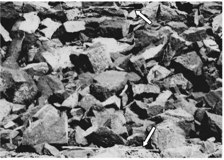
After every blast, muckpile pictures were taken and the images captured from the pictures were analyzed for fragment size distribution using the image analysis program. Three 10-ton truckloads of the muckpile were sieved for fragment size distribution. Figure1shows an image captured

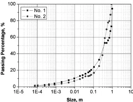
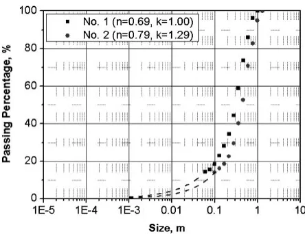
from a picture of a muckpile. The poles in the image were used to scale fragment particle size. Figure2 shows the fragment size distributions on a log-lin plot obtained by the sieving analyses. The mean particle size, D50, was 0.370 m for No. 1 blast and 0.360 m for No. 2 blast. Figure3 shows the fragment size distribution in Fig.2 plotted on alog-log plot. Note that in the region below the size about 0.04 m, the plots represent a straight line. Figure4 shows the analyzed fragment size distributions on a log-lin plot obtained with the image analysis program. The mean particle size, D50, was 0.346 m and 0.493 m, and the minimum particle size was 0.028 m and 0.014 m, respectively. In this study, the mini-mum particle size is denoted as the maximini-mum fines size. The average maximum fines size was therefore 0.020 m.

2.3 Evaluation of fines and the correction of fragment size distribution for the fines

When the results of sieving analysis were compared with those of image analysis, it was realized that there were some differences between the two distributions and the size distribution by image analysis did not contain particles with sizes less than about the average maximum fines size. We could therefore guess that the results of image analysis

needed to be corrected with respect to the fines less than the average maximum fines size. To estimate the ratio of the fines, sieved fragment size distributions (Fig.2) were averaged as shown in Fig.5 and compared with the distributions obtained by image analysis with assumption that the muckpile images did not include any fine material. In Fig.5, the mean particle size, D50, is 0.365 m. Considering that the average maximum fines size is 0.020 m, it was recognized that the ratio of the fines was 13%. That is to say, the size distributions obtained by image analysis did not contain the fines ratio of 13%. It was therefore clear that the size distributions by image analysis needed correction to consider the ratio of the fines. Considering that the distribu-tion curve of small particle size below 0.04 m was a straight line as shown in Fig.3, Gaudin-Schuhman distribution that shows a straight line on alog-logplot was adapted to plot the size distribution curve of the fines as:4)

Passing percentage for fines (%)¼ x k

n

100 ð1Þ

where x and k denote the size and the top size of the fragmented rocks, respectively, and n is the material constant.

The corrected size distribution and the size distribution of

Fig. 2 Fragment size distributions obtained by sieving analysis.

Fig. 3 Fragment size distributions obtained by sieving analysis on alog -logplot.

Fig. 4 Fragment size distributions obtained by image analysis.

the fines did not match as one smooth curve. Hence, we tried to find a matching point for a smooth transition between the two distribution curves and it was found that the passing percentage of 14% gave a good transition as one curve. As a result, the corrected distributions were smoothly connected with the size distributions including the fines ratio of 13% as shown in Fig.6. Here the average mean particle size, D50av, is 0.375 m and the dotted lines denote the size distribution for the fines. The average mean particle size became closer to the mean particle size obtained by sieving analysis, 0.365 m, moreover the modified fragment size distribution curves became closer to the fragment size distribution curves in Fig.2. It is important that the approaches for correcting fragment size distribution with the evaluation of fines make it possible to predict a realistic fragment size using image analysis. However, the ratio of the fines may be varied according to explosive type, rock type and so on and sieving analysis for various blasting type in various field may be required to obtain a general expression of fine-distribution. For these reason, it was required to develop an approach for estimating fragment size distribution with the evaluation of fines by the other ways. This paper therefore suggests a numerical simulation method to predict rock fragment size distribution with the evaluation of fines in bench blasting in the next section.

3. Numerical Rock Fragmentation

3.1 Numerical simulation method

Rock is generally treated as a heterogeneous material. The rock models for analysis therefore need to consider the scatter of strength, and rock strength can be expressed by Weibull’s distribution function5) with the assumptions that material fracture is governed by latent cracks and the hypothesis of the weakest link holds. The probability function with the tensile strengthtin volumeis then written in the following form:

Pð; tÞ ¼1exp

0

t

tð0Þ

m

m 1þ1 m

ð2Þ

where is the gamma function, m is the coefficient of homogeneity,0 is the reference volume and tð0Þdenotes the average tensile strength in the volume0.

ratio of normal stress and the tensile strength at the element boundary. If the fracture potential is greater then 1, the node between the two elements is separated into two nodes. To consider the fracture process zone in front of the crack tips, the approximate function of the tensile softening curve in rock fracture mechanics, which is the 1/4 model, was used.6) The Mohr-Coulomb fracture criterion was used to model the compressive fracture of the rock around the blast holes and the strength of the post-fractured element was modified so that the elements fractured could not have any tensile strength.6)

The JWL equation of state has been extensively used to describe isentropic expansion of detonation products. The equation forPas a function ofV at constant entropy can be written as;

P¼AexpðR1VÞ þBexpðR2VÞ þCV ð!þ1Þ ð3Þ

where A¼87:611(GPa), B¼0:0798(GPa), C¼

0:0711(GPa), R1¼4:30566, R2¼0:89071 and !¼0:35 (for ANFO explosive).7)P is pressure andV is the relative volume.

3.2 Numerical simulation results

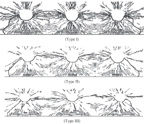
Figure7illustrates a schematic view of large-scale bench blasting. The analysis model has a free face, continuous boundary and charge holes parallel to the free face and the diameter of all the models is 200 mm. Three models were used for this study. For Type I, the burden and spacing were 2 m and 4 m, for Type II, 3 m and 6 m and for Type III, 4 m and 8 m, respectively. The properties of the models are listed in Table1. Figure8shows that the distribution of maximum principal stress and crack propagation as results from Type II

Fig. 6 Modified fragment size distributions.

explain well what phenomena happen in bench blasting before throw of the fragmented rocks begins. It also shows numerous radial cracks generated by tangential tensile stress. Radial cracks between the free face and the blast holes are particularly well developed. It is reasoned that the rock mass swelling at the free face generated tensile stresses perpendi-cular to the free face and returning tensile waves increased the magnitude of the tensile stresses at the tips of those cracks, while there are any cracks around the blast holes. Here the non-crack zone corresponds to a compressive fracture zone. This agreed with Persson’s assertion2)that the region near the blast hole is fractured without cracks and that radial cracks are generated in the outer region. Rock spalling caused by Hopkinson’s effect appeared only near the free face at all the three models. It agrees with Sassa’s results1) that the tensile stress caused by Hopkinson’s effect appeared only near the burden.

3.3 Numerical fragment size distributions

For image analysis, a fractured region is properly selected for each model, except for the compressive fracture zones, and the selected region is delineated and analyzed for fragment size distribution using the image analysis program. Figure9shows the image captured for the results from three Types. Considering that fragments are formed from crack propagation and coalescence, it may be assumed that the regions in the lines are to be the fractured rock due to blasting. The selected regions in Fig. 9 were delineated by using the delineation function of the Wipfrag image analysis program, which uses automatic algorithms to identify individual blocks of fragments using state of the art edge detection.8) Figure10 shows the delineation results.

Table 1 Properties of analysis model.

Average Compressive Strength (MPa) 75

Average Tensile Strength (MPa) 5

P-Wave Velocity,Vp(m/s) 2000

S-Wave Velocity,Vs(m/s) 1200

Density,(kg/m3_{) 2700}

Elastic Modulus,E(GPa) 9

Poisson’s Ratio 0.25

Fracture EnergyGf(Pam) 300

Coefficient of uniformity,m 5

Fig. 8 Maximum principal stress and crack propagation (Type II).

Fig. 9 Images captured from the simulation results.

Ratio of fine (%)¼ Compressive fracture area

Compressive fracture areaþDelineated area

100 ð4Þ

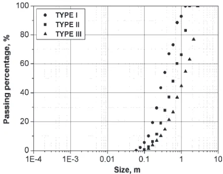
The fines ratio is added to the size distributions of the delineated zone. For plotting the size distribution of the fines, the Gaudin-Schuhman distribution was used. The distribution curves of the fines were connected with the distribution curves of the delineated area for each model. The numerical fragment size distributions considering the fines ratio are plotted as log-lin size distribution in Fig. 12. The dotted lines denote the size distribution for the fines. The ratios of the fines are 15%, 13% and 9%, the mean particle sizes, D50, are 0.25 m, 0.50 m, and 1.00 m and the top sizes of fragmented rocks are 1.29 m, 1.67 m and 2.78 m for Type I, Type II and Type III, respectively. In this figure, it is observed that the passing weight percentage of the size and the maximum passing weight percentage of the fines decrease with increases in the scale of burden and spacing, while the mean particle size increases with increase in the scale of burden and spacing, and the curves are approximately parallel to each other. When compared with experimental fragment size distributions, the distribution characteristics of the Type I

model was the closest to the experimental fragment size distributions in Fig.2. From these results, we could validate the correction method of numerical fragment size distribu-tions for fines.

Finally, it is worth noting that the numerical simulation method proposed does not predict a realistic fragment size distribution but also evaluates the ratio of fines according to the scale of burden and spacing in bench blasting.

4. Discussion

In Fig. 11, the mean particle sizes of the fragment size distribution increase with increase in the scale of the burden and spacing and the distribution curves are different with each other. After the correction of the fragment size distribution with evaluation of fines, the mean particle sizes of the fragment size distribution increase with increase in the scale of the burden and spacing and the curves are approximately parallel to each other as shown in Fig.12. It was recognized that these trends were coincident with the experimental results9)that the mean particle size shifts with the excavation method, but their distribution curves were parallel to each other in rock fragmentation. It is also expected that the correction approach with the evaluation of fines in Section 2.3 is applicable to a correction of image analysis results from a blasting in other rock type.

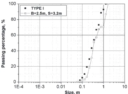
Figure13 shows the simulation result of Type I0 _model

(B¼2:5m,S¼3:2m). The Type I0_{model have the value of}

Fig. 11 Numerical fragment size distributions by image analysis.

Fig. 12 Numerical fragment size distributions with the correct evaluation

SB, 8.0 and the ratio ofS=B, 1.28. When compared to the fragment development of the Type I in Fig. 8, it was realized that more boulders were produced between the blast holes and the free face from the Type I0_{. The fragment size}

distributions of the Type I and Type I0 _{were compared as}

shown in Fig.14. D50 was 0.35 m and the top size was 1.67 m for Type I0_{. The ratio of fines of Type I}0_{was equal to}

that of Type I. Although the Type I0_{kept the same area and}

was pressurized with the same loading density as the Type I, the fragment size distribution became coarser. It is reason-able results because the Type I is close to wide-spacing blasting pattern, while the model is general bench blast pattern. The wide-spacing blasting method was developed to produce considerable benefits in term of better fragmenta-tion, less secondary blasting.10) It is expected that the numerical simulation method proposed would be applied to the design of blasting pattern to control a fragmentation.

It is well known that blast-induced fractures are generated by stress waves, and then under the action of the gas pressure, the fractures extend further. The numerical simulation method proposed in this study did not, however, considered the gas pressurization. Although this limitation would not have a large effect on the fragmentation characteristics, for realistic modeling, the simulation method should overcome these limitations. In addition, for more realistic modeling, the simulation method should consider geological discontinu-ities.

5. Conclusions

To evaluate fines in bench blasting, two bench experiments were conducted in the field and fragment sizes of blasted rocks were estimated by sieving analysis and image analysis.

The fragment size distributions by image analysis were corrected with the evaluation of the fines. From experimental results, it was found that the size distributions obtained by image analysis did not contain the fines ratio of 13%. After correct evaluation of the fines, the modified fragment size distributions were approximately coincident with the frag-ment size distributions obtained by sieving analysis and the average mean particle size became closer to the mean particle size obtained by sieving analysis.

A numerical simulation method to predict rock fragmenta-tion and verify the fracture mechanism in bench blasting was proposed. To determine the fragment size distributions from the results of the numerical simulation, a procedure using image analysis was suggested. The fragment size distribu-tions were corrected with the evaluation of fines, which correspond to a compressive fracture zone around a blast hole. As result of numerical simulation results, the ratios of the fines are 15%, 13% and 9%, the mean particle sizes, D50, are 0.25 m, 0.50 m, and 1.00 m and the top sizes of fragmented rocks are 1.29 m, 1.67 m and 2.78 m for Type I, Type II and Type III, respectively, and it is realized that the mean particle size increases with increases in the scale of bench blast model and the fragment size distributions approximately parallel each other.

Finally, this study showed the possibilities of realistic prediction of fragmentation using a numerical simulation method and image analysis and of determining rock fragmentation reasonably corresponding to the results of sieving analysis using image analysis with the correct evaluation of fines.

REFERENCES

1) K. Sassa and I. Ito: Trans. Soc. Min. Eng.235(1966) 167–178. 2) P. A. Persson, N. Lundberg and C. H. Johanson: Proc. 2rd Congress

I.S.R.M (1970) 353.

3) A. Minchinton and P. M. Lynch: Int. J. Blasting and Fragmentation1 (1997) 41–57.

4) R. Schuhmann: Am. Inst. Min. Met. Eng. (1941) 1189. 5) B. Epstein: J. App. Phys.19(1948) 140–147.

6) K. Kaneko, Y. Matsunaga and M. Yamamoto: J. Jpn. Exp. Soc.58 (1995) 91–99.

7) H. Hornberg and F. Volk: Prop. Exp. Pyro.14(1989) 199–211. 8) N. H. Maerz, T. C. Palangio and J. A. Franklin: Proc. Fragblast5

Workshop on Measurement of Blast Fragmentation (1996) 91–99. 9) W. Chen, K. Fukui and S. Okubo: Proc. 4th North Am. Rock Mech.

Symp. (2000) 27–32.

10) U. Langefors and B. Kihlstrom:The modern technique of rock blasting, (John Wiley & Sons, Inc., Stockholm, 1963).