Regularisation, interpolation and visualisation of diffusion tensor images using non Euclidean statistics

The Version of Record of this manuscript has been published and is available in Journal of Applied Statistics 23 September 2015 http://www.tandfonline.com/doi/10.1080/02664763.2015.1080671

Regularisation, interpolation and visualisation of diffusion

tensor images using non-Euclidean statistics

Diwei Zhoua

, Ian L. Drydenb

, Alexey A. Koloydenkoc_∗

, Koenraad M.R. Audenaertc

, and Li Baid

a

Department of Mathematical Sciences, Loughborough University, Loughborough, Leicestershire, LE11 3TU, UK;b

School of Mathematical Sciences, University of Nottingham, Nottingham, NG7 2RD, UK;c

Mathematics Department, Royal Holloway, University of London, Egham, Surrey, TW20 0EX, UK;d

School of Computer Science, University of Nottingham, Jubilee Campus, Nottingham, NG8 1BB, UK

(Received 7 February 2013; revised 16 December 2013, 31 December 2014, 11 April 2015; accepted 4 August 2015)

Practical statistical analysis of diffusion tensor images is considered, and we focus primarily on methods that use metrics based on Euclidean distances between powers of diffusion tensors. First we describe a family of anisotropy measures based on a scale invariant power-Euclidean metric, which are useful for visualisation. Some properties of the measures are derived and practical considerations are discussed, with some examples. Second we discuss weighted Procrustes methods for diffusion tensor interpolation and smoothing, and we compare methods based on different metrics on a set of examples as well as analytically. We establish a key relationship between the principal-square-root-Euclidean metric and the size-and-shape Procrustes metric on the space of symmetric positive semi-definite tensors. We explain, both analytically and by experiments, why the size-and-shape Procrustes metric may be preferred in practical tasks of interpolation, extrapolation, and smoothing, especially when observed tensors are degenerate or when a moderate degree of tensor swelling is desirable. Third we introduce regularisation methodology, which is demonstrated to be useful for highlighting features of prior interest and potentially for segmentation. Finally, we compare several metrics in a dataset of human brain diffusion-weighted MRI, and point out similarities between several of the non-Euclidean metrics but important differences with the commonly used Euclidean metric.

Keywords:anisotropy; metric; positive definite; power; Procrustes; Riemannian; smoothing; weighted Fr´echet mean;

Classification codes: 62G05; 62H11; 62H35; 62P10

1. Introduction

Diffusion tensor imaging (DTI) is an advanced magnetic resonance imaging (MRI) modal-ity which provides a unique insight into tissue structure and organisation in vivo. DTI has been applied to the study of brain diseases such as multiple sclerosis, schizophrenia, and stroke [25], and white matter tractography [4] is a useful application of DTI for investigating brain connectivity.

There has been substantial interest in the development of approaches for diffusion tensor processing. For example, a regularisation scheme was proposed to process a

sor field using diffusion direction maps and diffusion anisotropy maps [10]. A k-means algorithm with the Mahalanobis distance has been proposed for clustering tensors in the thalamus [40]. The Euclidean metric was used in level set segmentation methods [38, 45] for grouping tensor data of particular interest. However, the usual Euclidean method may be unsatisfactory for diffusion tensors due to the non-Euclidean nature of the diffusion tensor space. A potential drawback of using the Euclidean distance may be a violation of the positive semi-definiteness, e.g. in the course of extrapolation [2]. Also, Euclidean averaging is prone to swelling, i.e. inflation of the tensor determinant. To overcome this problem, several non-Euclidean approaches were developed. The affine-invariant Riemannian [5, 14, 30] and log-Euclidean Riemannian [2] metrics have been proposed for diffusion tensor smoothing and interpolation.

Procrustes analysis is another promising non-Euclidean approach to diffusion tensor processing [11, 43]. The full Procrustes shape metric is also invariant under scaling of the individual tensors, and the Procrustes metrics can deal with rank-deficient tensors unlike the affine-invariant and log-Euclidean Riemannian metrics [11]. This is further elaborated in the paper.

Thus, this paper focuses on weighted mean tensor processing using power-Euclidean and Procrustes based distances. DTI and weighted tensor averaging are briefly reviewed, and we also develop a family of anisotropy measures, which is useful for visualising different aspects of structure in DT images. As already mentioned, it is of both theoretical and practical interest to compare tensor processing methods based on different metrics. For example, it is valuable to know that the Euclidean average preserves the trace and hence the mean diffusivity (MD) [29], whereas the affine-invariant and log-Euclidean Riemannian metrics instead preserve the determinant, and hence the geometric mean diffusivity (GMD) [2]. We also compare in this paper various properties of our methods, focusing on the (principal-)square-root-Euclidean member of the power-Euclidean family of metrics and the Procrustes size-and-shape metric. While tensor processing methods based on these metrics can sometimes give very similar or identical results, we attempt to explain how the two metrics differ and what consequences their differences have for tensor processing. In particular, we both prove analytically and show by simulation that the two approaches can be radically different when used for processing of degenerate tensors. Thereby, it is established that unlike its Euclidean sibling, the Procrustes averaging preserves matrix ranks, i.e. dimension of diffusion.

More recently, it has been argued that a certain degree of swelling may be acceptable to compensate for Johnson (Rician) noise, and that the above Riemannian methods may therefore be biased in such scenarios [29]. We show here that the Procrustes metric and the square-root-Euclidean metric reduce the Euclidean swelling effect less aggressively than do the aforementioned Riemannian methods. This makes the Procrustes and square-root-Euclidean methods interesting alternatives when some swelling may indeed need to be allowed. A full comparison of the interpolated mean diffusivity under the two Riemannian, Procrustes, and all power-Euclidean metrics is also presented analytically, and illustrated empirically.

We also establish a key relationship between the Procrustes and square-root-Euclidean metrics in the form of an analytic bound, which is also illustrated on synthetic examples. We then also discuss a weighted regularisation model which incorporates smoothing and a generalised regularisation that forces the tensor field to favour a prescribed diffusion profile. The power-Euclidean and Procrustes metrics are again our main interest, and we discuss properties of the different methods using synthetic examples and human brain DT images.

Although the paper focuses on 3_×3 matrices, all our theoretical results also hold true for the general n_×ncase, even when this is not explicitly stated below.

2. DTI and anisotropy

2.1 Diffusion tensor imaging

Diffusion MRI yields quantitative measures reflecting the directions of water diffusion in white matter fibre tracts [35]. DTI assumes that a water molecule displacement x_∈R3

over a fixed time tin a voxel follows a zero-mean multivariate Gaussian distribution [1] with covariance matrix 2Dt, whereDis the diffusion tensor, which is a symmetric positive semi-definite matrix. We will write Ω_≥0(n) for the set ofn×nsuch matrices. Some of our discussion will be restricted to symmetric positive definite matrices, and we will write Ω>0(n) for the set of n×n such matrices; n = 3 is our main case here. The diffusion tensor at each voxel can be estimated from diffusion MR images [6, 23, 24, 42]. The eigensystem of the diffusion tensor plays an important role in DTI studies. Thus, the MD of the voxel is defined as

MD(D) = 1

3trD=

λ1+λ2+λ3

3 ,

where λ1 ≥ λ2 ≥ λ3 ≥ 0 are the eigenvalues of D. Whenever λ1 > λ2, the principal eigenvector is defined as the one corresponding to λ1 and is thought to be aligned with the dominant fibre orientation at the voxel. In biological tissues there are barriers such as cell walls and nerve fibres, and so it is easier for water molecules to diffuse along certain preferred directions. The dominance of the preferred direction of water molecule diffusion can be captured quantitatively using diffusion anisotropy measures [25, 39]. Fractional anisotropy (FA) is the most popular such measure [22], defined below as the proportion of the ‘magnitude’ of D that can be ascribed to anisotropic diffusion:

FA(D) =

v u u

t3

h

λ1−¯λ2+ λ2−λ¯2+ λ3−λ¯2

i

2 λ2₁+λ2₂+λ2₃ = s_λ

p

λ2, where ¯λ= MD(D) andλ2 ₌P3

i=1λ2i/3, andsλ is the sample standard deviation of the

spectrum of D ₆= 0, the zero tensor. FA ranges from 0 for complete isotropy to 1 for linear anisotropy, and planar diffusion (λ1 =λ2 > λ3 = 0, i.e. oblate diffusion ellipsoid) has FA(D) = 1/√2.

Procrustes anisotropy (PA) is an alternative anisotropy measure that has been pro-posed based on the full Procrustes metric [11], and is defined as follows:

PA(D) =

v u u u

t3

_√

λ1− √

λ2+√λ2− √

λ2+√λ3− √

λ2

2 (λ1+λ2+λ3)

= s

√

λ

√_¯

λ, (1)

where √λ= P3_i=1√λi/3 and s√_λ is the sample standard deviation of square roots of

2.2 A family of anisotropy indices

The power-Euclidean metric was briefly introduced in [11], and for a ₆= 0 (a < 0 is meaningful for full rank tensors only) is given by

dA(D1,D2|a) = 1 |a_| kD

a

1−Da2 k, (2)

where Da = EΛaET and EΛET is the spectral decomposition of D, and _kA_k2 = tr(ATA). As a _→ 0 the metric becomes the log-Euclidean metric dL(D1,D2) = klog(D1)−log(D2)k, which requiresD1 and D2 to be positive definite, i.e. ∈Ω>0(3).

We introduce another distance called the scale invariant power metric for a₆= 0 given by

dAS(D1,D2|a) = 1 |a_|

    

0 if D1 =D2=0

1 if eitherD1=0 or D2 =0

infβ∈RkβDa1− D

a 2 kDa

2k k otherwise,

(3)

which involves scaling of a powered tensor to best match a unit size powered tensor. Writing _hD1,D2i for the inner product tr(DT1D2) and assuming neither Di equals 0,

dAS(D1,D2|a) = _|1_a|

p

|sin(∠(Da

1,Da2))|. The angle ∠(Da1,Da2) is defined via its cosine cos(∠(Da₁,Da₂)) =_hDa₁,Da_2i/(_kDa_1kkDa_2k), which in the context of kernels [32] is known as the alignmentbetweenDa₁ and Da₂.

The anisotropy measure based on the scale invariant power-Euclidean metric with power ais a generalisation of FA given by

FA(Da) =

v u u

t3

h

λa_{1 −}λa2_{+ λ}a

2 −λa

2

+ λ3−λa

2i

2 λ2a

1 +λ22a+λ23a

= psλa

λ2a, (4)

where λa ₌P3

i=1λai/3 [11] and sλa is the sample standard deviation of the a-th power

of the eigenvalues of D. Note that

FA(Da) =_|a_|

r

3

2dAS(I3×3,D|a).

We see that FA(D) and PA(D) are both members of FA(Da_{) with a = 1 and a= 1/2}

respectively. Note that for any non-zero a, FA((cD)a) =FA(Da) for any constant c >0, i.e. all the members of this family of anisotropy maps are scale invariant. Perhaps less obvious is the following result that for any fixed tensor D, the family is monotonically increasing in a.

Theorem _{2.1 For any non-zero symmetric semi-positive definite D, FA(D}a_{) is an}

increasing function of a, where a_∈[0,_∞). For the proof, see Appendix A. Hence, we have

Note that as a_→0+, FA(Da) approximates a rank indicator function:

lim

a→0+FA(D

a_{) =}

    

0 if rank(D) = 3 1/√2 if rank(D) = 2 1 if rank(D) = 1.

Also

lim

a→+∞FA(D

a_{) =}

    

0 if λ1 =λ2=λ3 >0 1/√2 if λ1 =λ2> λ3 1 if λ1 > λ2≥λ3,

that is, any oblate tensor D in the limit flattens to a disk, whereas a general tensor becomes linear.

We can also define log-Euclidean Anisotropy (LA) for full rank tensors (apart from ones with λ1 =λ2 =λ3= 1) as follows

LA(D) = FA(log(D)) =

v u u u

t3

P3

i=1

log(λi)−log(λ)

2

2P3_i=1(log(λi))2

.

Note that LA(D) is not a member of the family (4), and FA(Da_{) does not converge to}

LA(D) asa_→0+. Hence the case of LA(D) is not covered by Theorem2.1, and indeed, for some tensors LA(D) _≤ FA(D) whereas for others LA(D) _≥ FA(D). Also, for any non-zero a, LA(Da_{) = LA(D), and by varying a, it is possible to make FA(D}a_{) smaller}

or larger than LA(D). Note also that as λ3 → 0 (while λ1 and λ2 are bounded away from 0 or vanish at slower rates), LA_→ 1. At the same time, as λ1 → ∞ (whileλ2 and λ3 are bounded or grow at slower rates), LA→ 1 as well. Thus, in the limit LA does not distinguish between planar diffusion and linear diffusion. Likewise, as λ1=λ2 → ∞ (whileλ3 is bounded or grows at a slower rate), LA→1/√2. Also, asλ2=λ3 →0 (while λ1 is bounded away from 0 or vanishes at a slower rate), LA→ 1/

√

2 as well. Thus LA in the limit does not distinguish between isotropic planar diffusion and linear diffusion either. These observations might also explain why FA and other members of its family (4) may be preferred in practice as elaborated in Section2.3 below.

At the same time, for full rank tensors,

lim

a→0+

FA(Da)

a =

v u u

t1

2 3

X

i=1

log(λi)−log(λ)

2

(5)

which is just the sample standard deviation of the spectrum of log(D), and is also GA(D)/√2, where GA is the geodesic anisotropy [9].

2.3 Practical comparisons of anisotropy measures

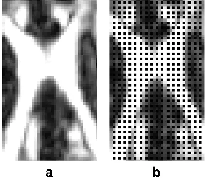
Figure 1. FA (a, a1) and PA (b, b1) maps; a and b are axial FA and PA maps; a1 and b1 are zoomed inset regions in the yellow box.

More generally, using values of a larger than 1 can increase the contrast in low anisotropy regions, while using values of a lower than 1, e.g. a = 0.5 as in PA, can increase the contrast in high anisotropy regions. It may then appear as if some bright-ness transformation of the [0,1] image intensity (anisotropy) range could increase the contrast within the bright structures of a1 to reveal the same amount of detail as in b1. However, for a general pair of anisotropy maps (a, b > 0,a ₆=b as in Theorem 2.1) such as FA (a= 1) and PA (b = 0.5), there need not exist a brightness transformation φ : [0,1]_→ [0,1] such that φ(FA(Da_{)) =FA(D}b_{) for all tensors D. In fact, consider D}

1 with eigenvalues [1,0.1,0.01] and D2 with eigenvalues [1,≈ 0.1011,0]. It is easy to see that both tensors have the same FA value of _≈0.9486, but FA(D0.025

1 )≈0.0864 whereas FA(D0₂.025) _≈0.7077, which would be impossible if φ as above existed. Therefore, com-puting FA(Da) for a range of a values is important for providing the end user with the flexibility of highlighting specific anisotropy ranges in real time and subsequently opti-mising the end user’s visual perception of specific features of the DT image. (Note that re-computing FA(Da_{) in real time for a range of avalues is not an issue.)}

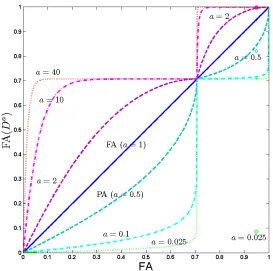
To illustrate the possibility of contrast adjustment with the help of the FA(Da) family of maps, Figure 2 presents FA(Da_{) maps of the following parametric family of tensors}

D(t):

D(t) =

                  

  

1 0 0 0 1 0 0 0 1₋2t

 

 if t_∈[0,1/2],

  

1 0 0

0 2₋2t0

0 0 0

 

 if t_∈(1/2,1]

for a _{∈ {40}1,₁₀1,1₂,1,2,10,40_}. Note that FA(D(0)) = 0, FA(D(1₂)) = √1

Figure 2. Members of the FA(Da_{) family of anisotropy maps are ordered as explained by Theorem 2.1 but}

still meet at the points of full isotropy (FA(Da_{) = 0), planar diffusion (FA(D}a_{) = 1/}√_{2) and linear diffusion}

(FA(Da_{) = 1). The isolated circles correspond to the tensorD}

1with eigenvalues [1,0.1,0.01], which has the same FA value of≈0.9486 asD2=D(t≈0.1011) (intersecting the curves at FA= 0.9486), whereas the other anisotropy measures (e.g.a= 1/2,1/40) disagree notably for these tensors.

3. Comparing distances

3.1 Weighted generalised Procrustes mean

We are often interested in weighted mean tensor estimation, for example when inter-polating or smoothing tensors. A brief description of the method was given in [44] but here we supply more details and consider more applications and results. Given a suitable distance functiond, the weighted Fr´echet mean [2,16] of a sample ofN diffusion tensors D1,...,DN is defined by

ˆ

Σ= arg inf

Σ N

X

i=1

wid2(Di,Σ), (6)

where the weights wi satisfy 0 ≤wi ≤1 and PNi=1wi = 1, and in applications can be,

for example, a function of the Euclidean distance from the location of interest to the sampling locations (e.g., voxels). Naturally, different choices of d(_·) generally result in different weighted mean diffusion tensors.

Procrustes analysis is a powerful shape analysis tool for matching configurations of points as closely as possible using the similarity transformations (rotation, translation and scaling) [12, 17]. In this study, a weighted Procrustes framework is proposed to compute the weighted Fr´echet mean tensor.

reflection while preserving scale. Thus, the Procrustes size-and-shape metric is defined as

dS(D1,D2) = inf

R∈O(3)kQ1−Q2Rk, (7)

where a 3_×3 rotation and reflection matrix R ranges over O(3), the space of 3_×3 orthogonal matrices. Note that dS in Equation (7) is well-defined as a metric on the

set of symmetric positive semi-definite matrices since QQT = PPT implies P = QR for some R_∈O(3) and the Frobenius (Euclidean) norm _{k · k} is rotation and reflection invariant.

Any orthogonal matrix ˆRthat minimises the norm of the difference in Equation (7) is given by ˆR=UVT, whereU,V_∈O(3) are obtained from a singular value decomposition QT₁Q2=V∆UT, with∆ a diagonal 3×3 matrix of singular values.

When a sample of N tensors is available, weighted generalised Procrustes analysis (WGPA) can be used to find the weighted mean ˆΣ when d(_·) = dS(·) is the

size-and-shape distance [11]. Specifically, WGPA computes ˆΣW GP A = ˆQW GP AQˆTW GP A, with

ˆ

QW GP A =PNi=1wiQiRˆi, where the orthogonal matrices ˆRi, i= 1, . . . , N minimise the

sum of weighted squared Euclidean norms given by

fW GP A(R1, ...,RN) = N

X

i=1

wikQiRi− N

X

j=1

wjQjRj k2

=

N

X

i=1

wik(1−wi)QiRi−

X

j6=i

wjQjRj k2

=

N

X

i=1

wi(1−wi)2 kQiRi−

1 (1₋wi)

X

j6=i

wjQjRj k2 . (8)

Note that Qi could be the Cholesky decomposition chol(Di) or the symmetric, i.e.

prin-cipal square root of Di or another choice such thatDi =QiQTi , since any two

decom-position matrices of the same tensor are related via an orthogonal transformation. We prefer the symmetric square root not least because its uniqueness extends to degenerate matrices. An iterative algorithm to minimise fW GP A was introduced in [44] and is used

here to produce experimental results in Section 6.2.

An extension of the method to a power Procrustes approach is where D =Q1/a, and Q =Da _{is the symmetric aroot. The algorithm proceeds exactly as above for an even}

power of 1/a, where above we have used 1/a= 2.

3.2 Other tensor distances and their properties

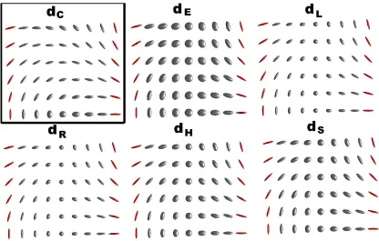
The weighted tensor averaging can be applied to interpolate between two diffusion ten-sors. Weighted averages of D1 and D2 corresponding to different metrics are listed in Table 1. The weights are typically constrained by w1 +w2 = 1, enabling us to write D(w) for D(1 ₋ w, w). For interpolation, we additionally require wi ≥ 0, i = 1,2,

but Table 1 does not make such assumptions. In the table, ˆR is the Procrustes min-imiser of Equation (7), and transposition in the case of dH is not necessary given

the symmetry of the principal square root tensors. The definitions of the metrics used in this table were summarised in [11]. Note that the Euclidean root distance dH(D1,D2) =kD11/2−D

1/2

Table 1. Weighted averages ofD1andD2 using different metrics.

Metric (notation) Weighted Average D(w1, w2) Euclidean (dE) w1D1+w2D2

log-Euclidean (dL) exp{w1log(D1) +w2log(D2)} Affine-invariant Riemannian (dR) D

w_{1 +}w₂

2

1

D−

1 2

1 D2D−

1 2

1

w2

D

w_{1 +}w₂

2

1 Cholesky (dC) [w1chol(D1) +w2chol(D2)]

[w1chol(D1) +w2chol(D2)]T Euclidean root (dH) (w1D11/2+w2D12/2)2

Procrustes size-and-shape (dS) (w1Q1+w2Q2R)(ˆ w1Q1+w2Q2R)ˆ T

All of the above interpolants D(w) satisfy d(D(w1),D(w2)) =_|w1−w2|d(D(0),D(1)) for all w1, w2 ∈ [0,1], and in particular describe the shortest path between D1 and D2 with respect to their metrics. We will refer to curves _{D(w), w_∈I _⊃[0,1]_} as geodesics through D1 and D2; extrapolation corresponds to woutside [0,1].

From their definitions, it is clear that dH(D1,D2) ≥ dS(D1,D2) for any tensors D1, D2. Since we find these two metrics particularly useful, especially when dealing with degenerate tensors, and often producing similar results in our studies, we want to un-derstand their relationship better. To this effect, we establish the following theorem.

Theorem _{3.1 Let D1,D2 ∈ Ω}

≥0(3). Then, √

0.5dH(D1,D2) ≤ dS(D1,D2) ≤ dH(D1,D2). Moreover, if D1 6= D2, and D1 and D2 are of rank 1, then √

0.5dH(D1,D2) < dS(D1,D2) and dS(D1,D2)/dH(D1,D2)→ √

0.5 as d(D1,D2)→ 0 in any metric d.

See Appendix Bfor the proofs of this and the following auxiliary result.

Proposition 3.1 LetQi,i= 1,2 be symmetric positive semi-definiten×nreal

matri-ces. Then

min

R∈O(n)kQ1−Q2Rk

2 _≥0.5kQ

1−Q2k2. (9)

Thus, in the rank 1 case, the two metrics diverge the most as the two tensors become indistinguishable. We also conjecture that in general, in order to approach the 1/√2 bound, the two tensors must become indistinguishable and simultaneously approach the subspace of rank 1 tensors; see Appendix B for more details. Section 4.3.2 below gives relevant supporting experiments.

Despite these seemingly rigid bounds, the two distances can lead to significantly dif-ferent results when used to average degenerate tensors, as established in the following proposition.

Proposition 3.2 Let rank(D1) = rank(D2)<3. Then rank(D(w1, w2)) is constant for all (general) w1, w2 ∈R, whereD(w1, w2) is as in the dS row of Table1.

of using dS in practice when dealing with positive semi-definite tensors.

It is worth noting that the Euclidean, log-Euclidean Riemannian, and the power-Euclidean metrics are all special cases of the following general type of metric

dg(D1,D1) =kg(D1)−g(D2)k. (10) Namely, letg be an injection from the non-negative real numbersR≥0 to the extended real line ¯R = _{{−∞} ∪}R∪ {+_∞}. Consider the extension of g to the following matrix function from Ω_≥0(3) to the 3×3 symmetric ¯R-valued matrices:

g(D) =E



g(λ01)g(λ02) 00

0 0 g(λ3)



ET,

where EΛET _{is the spectral decomposition of D.}

Thus, in the Euclidean case g(x) =x, in the log-Euclidean caseg(x) = log(x), and in the root-Euclidean case g(x) =√x.

We will refer to such metrics as Euclidean-based. In this case, the general weighted Fr´echet mean Equation (6) has a unique solution as shown below:

D(w1, w2) = arg min

D

w1d2g(D1,D) +w2d2g(D2,D)

D(w1, w2) =g−1(w1g(D1) +w2g(D2)), (11) which unifies the respective entries in Table 1above, and will be extended and exploited further in the ensuing discussion.

We would also like to understand how various tensor interpolations behave and com-pare in terms of the tensor size. For example, the swelling effect under the Euclidean averaging has been frequently mentioned in the literature. Although this effect is indeed straightforward, below we give its detailed mathematical explanation, which we have not seen stated explicitly in DTI literature. Namely, writing DE(w1, w2) for the weighted Euclidean average (with w1+w2 = 1,w1, w2 ≥0), the Minkowski Determinant Theorem [26] with dimension n= 3 gives

|DE(w1, w2)|

1

3 ≥w1|D1| 1

3 +w2|D2| 1

3 (12)

with the equality if and only if D2 = cD1 for some c ≥ 0. Thus, |DE(w1, w2)| ≥ min_{|D_1|,_|D_2|}, and if_|D_1|=_|D_2|but the tensors are distinct, the swelling is inevitable as_|DE(w1, w2)|>|D1|=|D2|for positive weightsw1, w2. Since both the affine-invariant and log-Euclidean Riemannian interpolations give_|DL,R(w1, w2)|=|D1|w1|D2|w2[2], the arithmetic-geometric mean inequality implies_|DL,R(w1, w2)| ≤ |DE(w1, w2)|[26] for any positive definite tensors D1 and D2 and for all (probability) weightsw1, w2.

A simple but useful observation is that the root-Euclidean determinants _|DH(w1, w2)| are sandwiched between the Euclidean _|DE(w1, w2)| and geometric, i.e. log-Euclidean and affine-invariant Riemannian, ones _|DL,R(w1, w2)|, as stated next.

Proposition 3.3 Letw1, w2be probability weights, and letD1andD2ben×npositive definite symmetric matrices, and letDL,R(w1, w2),DH(w1, w2), andDE(w1, w2) be their Riemannian (log-Euclidean or affine-invariant), root-Euclidean, and Euclidean weighted averages, respectively, where w1, w2≥0. Then we have

See Appendix D for the proof of this proposition and the following corrolary and proposition.

Corollary 3.1 Under the assumptions of Proposition3.3 above, we also have

|DL(w1, w2)| ≤ |DS(w1, w2)|.

We establish next that in general _|DS(w1, w2)| ≤ |DH(w1, w2)|, therefore

|DL,R(w1, w2)| ≤ |DS(w1, w2)| ≤ |DH(w1, w2)| ≤ |DE(w1, w2)|. (13)

Proposition 3.4 LetD1andD2ben×nsymmetric positive semi-definite real matrices, and let DS(w1, w2) and DH(w1, w2) be their Procrustes and root-Euclidean weighted averages, respectively, where w1, w2≥0. Then

|DS(w1, w2)| ≤ |DH(w1, w2)|.

We will see below that when D1 and D2 commute, DS(w1, w2) = DH(w1, w2). Our experiments in Sections 4.3.1 and 6.2 show further that _|DH(w1, w2)| dominates |DS(w1, w2)|by a relatively small margin only. This is not surprising given that compar-ison of the traces, or MDs, reverses the inequality as established next.

Proposition 3.5 For all D1,D2 _∈ Ω>0(3), and for all probability weights w1, w2, we

have

trDR(w1, w2)≤trDL(w1, w2)≤trDH(w1, w2)≤trDS(w1, w2)≤trDE(w1, w2). Moreover, the last two inequalities remain valid for allD1,D2 _∈Ω_≥0(3), and additionally we have

trDS(w1, w2)−trDH(w1, w2)≤0.5d2H(w21D1, w22D2). (14) See Appendix E for the proof. Even more is proved in [7], from which the following Corollary follows immediately.

Corollary 3.2 For any D1,D2 ∈ Ω≥0(3), trDA(w1, w2|a) is an increasing function of a_∈(0,_∞).

Also, for samples of N _≥2 tensors, we still have

trDL(w1, w2, . . . , wN)≤trDA(w1, w2, . . . , wN|a)≤trDE(w1, w2, . . . , wN),

for all a _∈ (0,1), and in particular for a = 0.5, which corresponds to the square root-Euclidean averaging.

Note that trDL(w1, w2) ≤trDE(w1, w2) has been, at least implicitly, commonly ac-knowledged in DTI literature (e.g. [2,29]); trDR(w1, w2)≤trDL(w1, w2) has also been mentioned (e.g. [2]). However, we have not seen the other inequalities stated explicitly in the DTI literature.

We also point out that the power-Euclidean interpolants satisfy tr(DA(w1, w2|a)a) = w1tr(Da1)+w2tr(Da2), so, for our main example ofa= 0.5, tr(DH(w1, w2)

1

w2trQ2. Thus, if D1 and D2 have equal traces of their square roots, then this will be preserved by the square root of the interpolant for all weights with w1+w2= 1.

Returning to the dominance of _|DH(w1, w2)|over |DS(w1, w2)|(Proposition 3.4), and in view of trDH(w1, w2) ≤ trDS(w1, w2), we note that the positivity of the difference |DH(w1, w2)| − |DS(w1, w2)|cannot be explained by the first-order approximation.

All in all, the Procrustes and root-Euclidean methods may be a good compromise as they do give some swelling (which is clear from Equation (12) withDi replaced byQi),

but their swelling is less aggressive than that of the Euclidean method. This may be helpful in view of [29] arguing that swelling may be desirable in certain scenarios.

Now, we consider a special situation of averaging an isotropic tensor with a general tensor, which is also illustrated by experiments in Section 4.3.1. Since this means that the reference tensorsD1 andD2 commute, the log-Euclidean Riemannian and the affine-invariant Riemannian averages will be identical [2], and we now show other implications of this assumption.

Proposition 3.6 Assume that one of the tensors D1, D2 (as in Table 1) is isotropic; without loss of generality, let it be D1, i.e. D1 = λI3_×3 for some λ ≥ 0. Let dg be a

Euclidean-based metric. Let λ1, λ2, λ3 be eigenvalues of D2,

(1) The weighted average tensor D(w1, w2) is given by Equation (15) below. Subse-quently, if g is increasing, then the orientation of D(w1, w2) is the same as the orientation of D2 for all weights with w2 6= 0. In particular, if λ1 > λ2, i.e. D2 is prolate (has a well-defined direction), then D(w1, w2) is also prolate and has the same direction (providedw2 6= 0).

(2) The Procrustes averaging is identical to the root-Euclidean averaging, andD(w1, w2) in this case is given by Equation (16) below.

(3) The (log-Euclidean or affine-invariant) Riemannian average tensorD(w1, w2) is given by Equation (17) below.

(4) D(w1, w2) for the Euclidean averaging is given by Equation (18) below.

(5) The Euclidean, log-Euclidean, the affine-invariant Riemannian, root-Euclidean, and the Procrustes interpolations all preserve the orientation ofD2, providedw26= 0.

E

_g−1_((w

1g(λ)+w2g(λ1)) 0 0

0 g−1_((w

1g(λ)+w2g(λ2)) 0

0 0 g−1_((w

1g(λ)+w2g(λ3))

ET, (15)

where EΛET is the spectral decomposition of D2 with eigenvaluesλ1 ≥λ2≥λ3.

Eλw2₁I3×3+w22Λ+ 2w1w2 √

λ√ΛET, (16)

E(λw1_Λw2_)ET_{, (17)}

E(λw1I3×3+w2Λ)ET. (18) The proof of this proposition is straightforward and is given in AppendixF.

Clearly, the above results, including the equality of the root-Euclidean and Procrustes averages, immediately generalise to any commuting tensors D1 and D2. However, it is understood that in general, eigenvalues of only one of the two tensors can be ordered at a time when generalising Equation (15) to Equation (19) below:

E

_g−1_((w

1g(γ1)+w2g(λ1)) 0 0

0 g−1_((w

1g(γ2)+w2g(λ2)) 0

0 0 g−1_((w

1g(γ3)+w2g(λ3))

whereγ1, γ2, γ3 are eigenvalues ofD1. Thus, the direction of the average tensor may turn out to be that of a non-principal eigenvector of D1 or D2.

Although we focus on interpolation, extrapolation outside the shortest path between D1 and D2 is easily included by relaxing the non-negativity constraint on the weights wi (see Section 4.3.2).

Finally, we note that other relevant metrics and more general measures of divergence continue to be proposed for symmetric positive definite matrices. One such example is the root Stein Divergence [34]

dStein(D1,D2) =

s

log det

1

2(D1+D2)

−1₂log det (D1D2), (20)

but we do not attempt to overview all such proposals in this paper.

4. Interpolation and smoothing

We now apply the above ideas and results on weighted averages to the tasks of interpo-lation and smoothing.

4.1 Choice of weights

The choice of weights is application dependent. For example, wi could be a decreasing

function of the Euclidean distance from the location of interest to the sampling location i. One simple choice for the weights is the inverse distance function given by

wi =

d−_i1

N

P

j=1 d−_j1

, i= 1, ..., N, (21)

wheredi is the Euclidean distance from the location (voxel) at which the weighted mean

is to be estimated, to the location (voxel) of ith tensorDi.

For more flexibility, the following exponential weight function is proposed and used in this paper:

wi=

exp(₋Ad2

i) +B N

P

j=1

[exp(₋Ad2

j) +B]

, i= 1, . . . , N, (22)

where A, B _≥0. The two parameter exponential weight family is flexible since it allows us to adjust the wi depending on the application, as seen in Section4.2where we discuss

cross validation.

Given distances di, i= 1,2, ..., N, some properties of exponential weight function are

listed below:

As A_→+_∞ and B = 0,

wi→

(

1/k if i_∈arg min_{d1, d2, ..., dN},

wherekis the size of the set arg min_{d1, d2, ..., dN}. Under any of the following conditions,

the weight distribution becomes uniform, i.e. wi → 1/N: (a) A → +∞ and B 6= 0 is

fixed; (b) A_→0 andB is fixed; (c) B_→+_∞ and Ais fixed.

4.2 Cross-validation

To illustrate how parameters A and B in the weight function (22) can be chosen in practice, and to also assess the weighted mean estimators, a cross-validation procedure is carried out over a region of interest shown in Figure 3(a) and taken from the real human brain data described in Section 6 below. Voxels V1,...,VK (K = 630 for this

example) shown in Figure 3(b) in black contain the validation tensors and remaining voxels contain training tensors. All tensors D1,..., DK are initially estimated using a

Bayesian framework [42] and the resulting estimates are considered the ground truth for the purposes of cross-validation. We re-estimate the tensor at voxel Vi, i = 1,...,K by

computing the weighted mean of its four first-order neighbours (i.e. tensors from two horizontally and two vertically adjacent voxels). The spatial resolution in the horizontal direction is twice that in the vertical direction, hence di in Equation (22) is taken to be 1

for horizontal neighbours and 2 for vertical neighbours, hence the weights are generally unequal.

To compare the effects of using the EuclideandE, log-EuclideandL, root-EuclideandH,

and ProcrustesdS distances in Equation (6), we compute the root mean square distance

(RMSD) between the re-estimated tensor Dcv

i and the original estimate Di, as shown

below:

RM SD(d) =

v u u

t 1

K

K

X

i=1

d(Di,Dcv_i )2,

where dcan be any suitable metric, such as dE,dL,dH, and dS.

Figure 3. A two-dimensional region of interest; locations of validation tensors are shown in black (b) against the background of FA map (a) of the same region (the remaining locations provide training tensors).

To choose parameters A and B (A >0, B >0) for the weight function (22), we con-siderRM SD(dE),RM SD(dL),RM SD(dH), andRM SD(dS) simultaneously. A greedy

and B = 0.01). We then first increase A in steps of 0.01 and calculate the RMSD val-ues. If at least one RMSD value starts increasing, the previous value of A is retained as optimal. Next, we increase B in steps of 0.01 and re-calculate all the RMSD values. If at least one RMSD value starts increasing, the previous B value is declared optimal. The optimal parameter setting for the example in Figure 3 is found to be A = 2 and B = 0.01. We choose to optimise over A first since this parameter has a bigger impact on the weights.

Table 2showsRM SD(dE),RM SD(dL),RM SD(dH), andRM SD(dS). The weighted

Procrustes approach provides the smallest RM SD(dE), RM SD(dH), and RM SD(dS)

measures in this example, whereas the weighted root-Euclidean method provides the smallest RM SD(dE) andRM SD(dL) andRM SD(dS) measures. Thus, in this example,

the two methods perform best in general, although their performances are very similar.

Table 2. Measures of the cross-validation results with different methods.

Euclidean log-Euclidean Euclidean root Procrustes

RM SD(dE) 0.00005 0.00006 0.00005 0.00005

RM SD(dL) 0.32601 0.31696 0.29664 0.29881

RM SD(dH) 0.00101 0.00094 0.00093 0.00092

RM SD(dS) 0.00082 0.00081 0.00077 0.00077

4.3 Interpolation and extrapolation

In Sections 4.3.1 and 4.3.2 below we consider the simplest case of interpolation and extrapolation of two tensors, respectively, using the main metrics of interest. Then, in Section 4.3.3we briefly illustrate the lack of invariance of the Cholesky interpolation to orthogonal changes of coordinates, and therefore its lack of practical application in DTI. This is followed by Section 4.3.4 with experiments on interpolation of four tensors.

4.3.1 Interpolation of two diffusion tensors

We illustrate the observations of Proposition 3.6and also investigate more general paths obtained with the metrics listed in Table 1. Specifically, we choose two reference tensors D(0) andD(1) and then interpolate between them by samplingN₋1 additional tensors along the shortest path as follows:

D(wi) = arg min D

(1₋wi)d2(D(0),D) +wid2(D(1),D)

, (23)

resulting in the total of N + 1 tensors with weights wi = i/N, i = 0,1, . . . , N. The

settings of D(0) andD(1) for each experiment are as follows:

Experiment I:

D(0) =4 0 00 4 0 0 0 4

, D(1) =87..50 750 8..50 050 0 0 0 4

=

1

√ 2 0−

1 √ 2 1 √

2 0 1 √ 2

0 1 0

16 0 0 0 4 0 0 0 1

1 √

2 0− 1 √ 2 1 √

2 0 1 √ 2

0 1 0

T

Experiment II:

D(0) =54..50 450 5..50 050 0 0 0 1

=

1

√ 2 0−

1 √ 2 1

√₂ 0 √1₂

0 1 0

10 0 0 0 1 0 0 0 1

1 √

2 0− 1 √ 2 1

√₂ 0 √1₂

0 1 0

T

,

D(1) =−411.72.46 36−11.28 0.46 0

0 0 4

=

_sin(

−0.1π) 0 cos(1.1π) cos(−0.1π) 0 sin(1.1π)

0 1 0

40 0 0 0 4 0 0 0 1

sin(−0.1π) 0 cos(1.1π) cos(−0.1π) 0 sin(1.1π)

0 1 0

T

.

To help us compare the effects of using the different metrics on the size, orientation, and shape of the interpolated tensor D(wi), we measure its volume (determinant |D(wi)|)

and perimeter (trD(wi)), angle φ(wi) of relative orientation, and fractional (FA) and

Procrustes (PA) anisotropies. The angle φ(wi) is the (non-obtuse) angle between the

direction (principal eigenvector pv(wi)) ofD(wi) and the direction (principal eigenvector

pv(1)) ofD(1):

φ(wi) = arcsin(kpv(1)×pv(wi)k)×180◦/π, i= 0, . . . , N. (24)

Experiment I, where D(0) is isotropic, illustrates the observations of Proposition 3.6. Since D(0) has no orientation, φ(0) is undefined in this case and will be replaced by limφ(w) as w_→0.

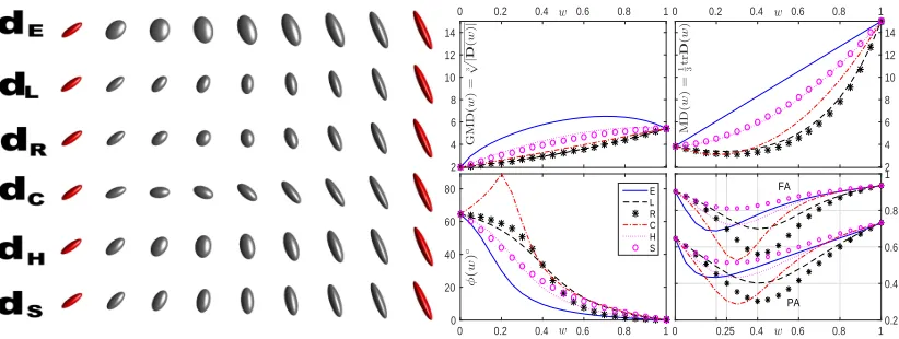
The left pane of Figure 4 shows six geodesic paths in Experiment I with N = 8. Unlike D(0), D(1) is strongly anisotropic in this experiment, and the two tensors have the same volume. The right pane displays the above measures of size, orienta-tion, and shape, using N = 20 for higher accuracy. The well-known swelling effect of the Euclidean interpolation is clearly seen from the plot of the GMD given by the cubic root of the determinant of D(wi). Further, in the case of Procrustes

interpola-tion (which is identical here to the root-Euclidean interpolainterpola-tion), Equainterpola-tion (16) gives D(wi) =E

4(1₋wi)2I3×3+wi2Λ+ 4wi(1−wi)

√

ΛET_.

Since D(1) is prolate (in the directionpv(1)), so is each interpolantD(wi), i.e.pv(wi)

aligns withpv(1) andφi= 0◦for alli= 1,2, . . . ,20, for all but the Cholesky interpolation

(the Cholesky method cannot be expressed in terms of matrix functions defined via the spectral decomposition) as promised by item (5) of Proposition3.6.

In the case of the log-Euclidean interpolation (which is identical here to the affine-invariant Riemannian interpolation), Equation (17) gives D(wi) =E 41−wiΛwi

ET. With the Cholesky metric (dC) the angleφ(wi) decreases gradually from about 15.5◦

(φ(w1 = 0.05)) to 0◦ (φ(w20 = 1)) along the geodesic path. It is worth recalling that the Cholesky metric is problematic in practice due to its lack of invariance to orthogonal transformations.

Since the log-Euclidean and affine-invariant Riemannian methods provide the same monotonic geometric interpolation of determinants (even when their geodesics are oth-erwise distinct) _|D(w)_| = _|D(0)_|1−w_|D(1)_|w, _|D(0)_| = _|D(1)_| implies that these meth-ods preserve the volume and subsequently GMD along their geodesic [2], whereas the other methods result in some swelling. The Euclidean averaging instead gives monotonic linear interpolation of traces trD(w) = (1₋w) trD(0) +wtrD(1) (which, provided trD(0) = trD(1), preserves the trace and subsequently the MD) [29]. The GMD and MD plots also illustrate the dominance of the arithmetic mean over the geometric mean, as well as the general inequality (13) and Proposition 3.5, respectively.

inter-polants, which in turn dominate the non-Euclidean Riemannian interpolants. The same ordering holds for the PA graphs, whose differences are even less noticeable in this exam-ple. Note that this ordering is not general, and, for example, increasingλ(the eigenvalue of D(0)) to 6 reverses this order, and setting λ= 5 makes the distinct FA (PA) curves cross (not shown). Note also that for the non-Euclidean Riemannian interpolants we have FA(D(w)) =FA(Λw); in particular, PA(D(1)) =FA(D(0.5)) for this geodesic.

Thus, the root-Euclidean/Procrustes geodesic disturbs the shape slightly more than does the log-Euclidean and affine-invariant Riemannian geodesic, but still notably less compared with the Euclidean geodesic.

w

0 0.2 0.4 0.6 0.8 1

G M D ( w ) = 3 p | D ( w ) | 4 4.5 5 5.5 6 6.5 7 w

0 0.2 0.4 0.6 0.8 1

M D ( w ) =

1tr3

D ( w ) 4 4.5 5 5.5 6 6.5 7

0 0.2 0.4 0.6 0.8 1

φ ( w ) ◦ 0 5 10 15 E L R C H S

0 0.2 0.4 0.6 0.8 1 0 0.2 0.4 0.6 0.8 1 FA PA w w w w

Figure 4. Experiment I: geodesic paths between two tensors of the same volume (red). Tensor D(0) (left) is fully isotropic and tensorD(1) (right) is strongly anisotropic. The geodesic paths are obtained withdE(),dL(),

dR(), dC(), dH() anddS(). As explained by Proposition3.6,dH anddS yield the same results here; likewise,

the results from usingdLand dR are the same in this case [2]. (φ(0) is undefined and replaced by limφ(w) as

w→0). The GMD and MD of the different interpolants compare according to Inequality (13) and Proposition3.5, respectively. The non-Euclidean Riemannian interpolants satisfy FA(D(w)) =FA(Λw) in this example, implying PA(D(1)) =FA(D(0.5)) for this geodesic.

In Experiment II, tensorsD(0) and D(1) are neither orthogonal nor collinear, and are of different shapes and sizes. Figure 5 shows six distinct geodesic paths between D(0) and D(1). The Euclidean metric again suffers significant swelling. The geometric (log-Euclidean and affine-invariant Riemannian) interpolation of the determinants (_|D(w)_|= |D1|1−w|D9|w) yields the lowest volume evolution among the considered methods. The Cholesky interpolation gives slightly larger volumes. The Procrustes determinant (GMD) curve is uniformly and notably above these three, and it is dominated, albeit less notably, by the root-Euclidean determinants.

The Cholesky path has a significant cusp (nearly 90◦_{) in the orientation in this}

ex-ample. The Euclidean orientational angle curve is everywhere dominated by the others except for the affine-invariant Riemannian one, which it crosses on approach to D(1). Orientational angle curves of the non-Euclidean methods intersect non-trivially; the log-Euclidean and affine-invariant Riemannian curves tend to dominate the root-log-Euclidean and to a lesser extent the Procrustes orientation curves. The log-Euclidean and affine-invariant Riemannian orientation curves clearly reveal a sigmoidal shape, which is more pronounced in the affine-invariant case.

In summary, the Procrustes size-and-shape metric and to a lesser extent the Euclidean root metric offer overall least variable interpolations of the size, orientation and shape.

w

0 0.2 0.4 0.6 0.8 1

G M D ( w ) = 3 p | D ( w ) | 2 4 6 8 10 12 14 w

0 0.2 0.4 0.6 0.8 1

M D ( w ) =

1tr3

D ( w ) 2 4 6 8 10 12 14 w

0 0.2 0.4 0.6 0.8 1

φ ( w ) ◦ 0 20 40 60 80 E L R C H S w

0 0.25 0.4 0.6 0.8 10.2

0.4 0.6 0.8 1 FA PA

Figure 5. Geodesic paths in Experiment II between two general reference tensorsD(0) (left, red) andD(1) (right, red) with general (i.e. non-collinear non-orthogonal) orientation, different shape and size. The geodesic paths are obtained withdE(),dL(),dR(),dC(),dH() anddS(). The Geometric and Arithmetic Mean Diffusivities of the

different interpolants compare according to Inequality (13) and Proposition3.5, respectively. PA helps resolving ambiguity of FA atw= 0.25 where FA of the Euclidean and affine-invariant interpolants coincide, but their PA values do not. There is no general ordering of anisotropies apart from the log-Euclidean interpolants dominating the affine-invariant ones [2].

From the examples discussed above, and several more in [41] and other related studies (e.g. [2]), it does seem that the Euclidean metric may be very problematic, especially due to the swelling of the determinant (apart from situations where a certain degree of swelling may help compensate for a previously suffered shrinkage [29]).

That the Cholesky metric should never be used in the standard DTI setting due to its lack of orthogonal invariance is illustrated in Section 4.3.3 below, and the above experiments also highlighted other potential issues with this metric. The log-Euclidean and affine-invariant Riemannian metrics generally give similar geodesic paths [2], and have a small advantage in Experiment I. The Procrustes size-and-shape and Euclidean root metrics offer similar interpolated tensors, and they are preferable in Experiment II.

4.3.2 Rank deficiency and extrapolation

The log-Euclidean and affine-invariant Riemannian metrics, as well as the root Stein Divergence (20) all give infinite distances between any positive definite tensor and any degenerate tensor. Furthermore, such metrics are undefined if both the tensors are rank-deficient. Therefore, when working with rank-deficient tensors, the root-Euclidean and Procrustes metrics may be advantageous. Generally, dH(D1,D2) and dS(D1,D2) give similar results, however, their (relative) disagreement tends to its supremum (dH/dS =

√

2) when the tensors become indistinguishable and simultaneously approach the rank 1 subspace; see also Theorem 3.1above.

The potential advantage of the Procrustes size-and-shape metric when extrapolating towards rank-deficient tensors has been noted in [31] in the infinite dimensional case of covariance operators. Similarl to the geodesic through two covariance operators defined in [31], geodesics through two diffusion tensors with the Euclidean root metric and the Procrustes metric are given by DH(w) = DH(1−w, w) and DS(w) = DS(1 −w, w)

from the respective rows of Table 1, where the weights are no longer constrained to be non-negative, i.e. w_∈R.

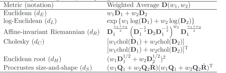
tensors, using dH and dS, and illustrating Proposition 3.2. The reference tensors are

defined as follows

D(0) =

 1 0 00 1 0

0 0 0



,D(1) =V

 2 0 00 1 0

0 0 0



VT_{,with V=}



−00.8391.5441 00..7040 04565 0..45652960 0 ₋0.5440 0.8391



.

The angle between the principal planes of these tensors is about 33◦, and the (2D) shapes of the tensors are also different: FA(D(0)) = 1/√2 _≈0.7071 (2D isotropy), and FA(D(1)) = 0.7746. Figure 6 shows dH(D(0),DH(w)) and dS(D(0),DH(w)) against

w _∈ [0,5]; the dH/√2 ≤ dS ≤ dH bounds are also illustrated. The difference between

dH and dS along the Euclidean root geodesic is hardly noticeable for w >3, whereas in

the case of the Procrustes size-and-shape geodesic the distances disagree more noticeably over the entire (0,5] range. Figure 7 shows the minimum eigenvalue λ1, determinant,

Figure 6. The Procrustes size-and-shape dS and the Euclidean root dH distances fromD(0) to the averaged

(interpolated or extrapolated) tensorD(w) along the Euclidean root geodesic (left) and the Procrustes size-and-shape geodesic (right).

and FA of DH(w) and DS(w) versus w ∈ (0,5). The Euclidean root geodesic yields

positive, albeit very small, λ1’s already in the course of interpolation (w_∈(0,1)). This would imply emergence of 3D diffusion from 2D diffusion, which may be hard to jus-tify from the viewpoint of physics. The minimal eigenvalue grows very rapidly in the course of extrapolation (w > 1). A similar behaviour is observed with the determinant |DH(w)|, even though it appears to be nearly zero forw∈(1,2], before a steep take-off

over w > 3. As explained in Proposition 3.2, the Procrustes geodesic does not suffer from this problem, i.e., it does not require full rank (3D) tensors to either interpolate or extrapolate through rank 2 tensors, which makes its action more realistic. Figure8shows the product λ1(w)×λ2(w) of the two largest eigenvalues, which exhibits the growth of the effective volume (area) ofDS(w) in its principal non-degenerate plane; the Euclidean

extrapolation in this Figure appears misleadingly regular while in reality it goes out of space Ω_≥0(3) (λ3(w)<0 for w >1).

its shape). FA of the Procrustes interpolations and extrapolations varies little, always remaining within the [1/√2,1) range of the planar diffusion. For larger w values, i.e w > 5, FA(DH(w)) may also be observed (not shown in the figure) to behave

non-monotonically, yet never rising back to the 1/√2 level of the planar diffusion. In summary,

Figure 7. Minimum eigenvalueλ3(left), determinant (middle), and FA (right) ofDS(w) (dotted line) andDH(w)

(solid line) versus the (interpolation [0,1] and extrapolation (1,5]) weightw.

both DH(w) and DS(w) expand in the course of extrapolation beyond D2 (w > 1), eventually becoming increasingly isotropic. However, DS(w) confines its expansion to its

principal plane (_|DS(w)|= 0 whileλS1(w)×λS2(w) grows).DH(w), on the other hand,

does not have this (λ3(w) = 0) constraint and expands in the entire 3D space.

w

0 1 2 3 4 5

λ1

∗

λ2

0 10 20 30 40 50 60 70 80 90

E H S

Figure 8. Product of the two largest eigenvalues ofDS(w) (dotted line),DH(w) (solid line), andDE(w) (dash

line) versus the (interpolation [0,1] and extrapolation (1,5]) weightw.

4.3.3 Interpolation under simultaneous rotation

It is known [11] that all of the metrics considered in this paper, exceptdC, are invariant

to orthogonal transformations of the underlying 3D space, i.e. d(UD1UT,UD2UT) = d(D1,D2) for allU∈O(3). This is very important in practice as any method for diffusion tensor processing must be independent of the choice of the reference frame [2]. Below we include a set of simple orthogonal change of frame experiments to demonstrate this issue.

Consider two mutually orthogonal tensors D(0) and D(1) with the same eigenvalues (40, 2, 1). Since the largest eigenvalue is much greater than the other two,D(0) andD(1) are nearly linear (and their principal eigenvectors are orthogonal); the corresponding ellipsoids are placed at the left and right top corners, respectively, of each of the six plots of Figure 9. Next, we simulate five orthogonal changes of the reference frame by rotating it by 15◦, 30◦, 45◦, 60◦, and 75◦ in the plane of view, so that the corresponding representations of UD(w)UT _{with w = 0 and w= 1 are placed (top down) in the left} and right most columns (red), respectively, of each of the six plots of Figure9. Each plot corresponds to one of the aforementioned metrics, and samples along the geodesic paths (rows) for each reference frame and each metric are defined according to Equation (23) with N = 8.

It can be seen, e.g. by looking at the middle ellipsoids of the top and bottom rows of the boxed plot, that the Cholesky geodesic paths are not invariant under the orthogonal transformations of the reference frame. Namely, the shape and size (determinant) of the interpolated tensor differ across the transformed geodesic paths. Although if viewed individually outside the change of frame context each of these Cholesky paths appears to be very reasonable, the lack of invariance renders the method unreliable in practice. The other metrics, as expected, give invariant geodesic paths, which are also included in this figure for the sake of completeness of the demonstration.

4.3.4 Interpolation of four tensors

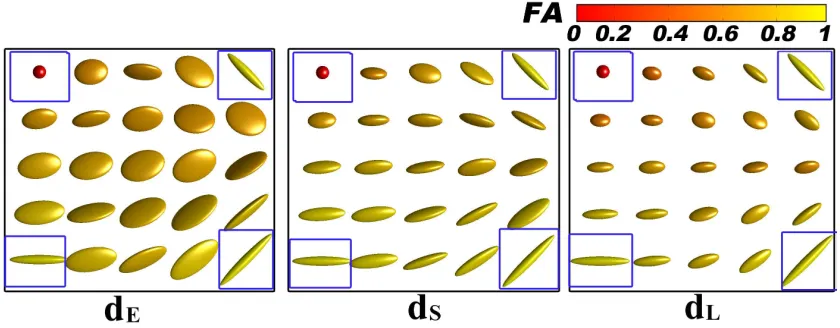
The next experiment is to interpolate in a 2-dimensional region. Specifically, we mesh the region with a regular 5_×5 grid, and place four synthetic tensors D1,1,D1,5,D5,1,D5,5 at the corners of the grid. At each of the 21 remaining nodes (i, j), a weighted average of these four tensors is computed according to Equation (6) and using the exponential weight function (22) withA= 2 andB = 0.01 (Section 4.2) and the Euclidean distances between the nodes of the grid in the definition of the weight function. Figure 10 shows results of the interpolations using the Euclidean, Procrustes and log-Euclidean metrics. At the top left corner, the diffusion tensor is isotropic (spherical) and of a small volume. Tensors at the other three corners are anisotropic with different volumes and orientations. The interpolated tensors from the Euclidean results have large volumes. Interpreting the Euclidean interpolation is also problematic in terms of the orientation and shape. The log-Euclidean interpolation tends to produce significantly smaller tensors. The Procrustes metric appears to provide a reasonable interpolation of the tensor volume, orientation and anisotropy.

Figure 10. Interpolation of four tensors at the corners of a grid. Left: Euclidean interpolation (dE). Middle:

Procrustes interpolation (dS). Right: log-Euclidean interpolation (dL). FA is used for the colouring of the tensors.

5. Tensor regularisation

In the following, we develop a weighted regularisation model which incorporates the smoothness of local diffusion and regularisation by imitation of a prescribed diffusion behaviour. Specifically, the Procrustes size-and-shape metric is adapted in the regulari-sation model.

5.1 Weighted regularisation model

Consider a sample of diffusion tensors D1, . . . ,DN from a noisy tensor field containing

N voxels with coordinates xi ∈Z3,i= 1, . . . , N. Now suppose we wish to regularise this

tensor field. We propose a weighted regularisation model, which is defined by minimising the following function with respect to Σj ∈Ω>0(3), j= 1, . . . , N,

f(Σ1,Σ2, . . . ,ΣN) = N

X

j=1

N

X

i=1

wijdp1(Di,Σj) +λ N

X

j=1

=

N

X

j=1

" _N X

i=1

wijdp1(Di,Σj) +λdq2(Π,Σj)

#

. (25)

Here the weightswij can be again obtained via some decreasing function of the Euclidean

distance betweenxi andxj(see Section4.1),p,q ≥0, andλis a regularisation parameter

(λ > 0), and Π is a reference tensor, representing the prescribed diffusion behaviour. Users can either define their own reference tensor with the expected diffusion profile or choose a representative tensor from the tensor field as a reference tensor. For a simple example, by employing a multiple of the identity tensor as the reference tensor we can regularise the tensor field to be both more isotropic and less variable in intensity. Note that d1 and d2 are general, i.e. can be non-Euclidean and need not be the same. When appropriate, Ω>0(3) can be replaced by Ω≥0(3).

The proposed regularisation model (25) simultaneously smooths each tensor Di,

i = 1, ..., N, by averaging it with its neighbours (endogenous regularisation) and also makes Di where i = 1, ..., N imitate the reference tensor (exogenous regularisation).

The flexibility of having a reference tensor can be exploited to introduce additional in-formation about the expected diffusion profile in the given region, or to highlight, and eventually segment, local structures. Allowing the end user to modifyΠ, e.g. by varying its spectrum and the Euler angles of the eigenvectors, in real time in a visualisation session might help pick up otherwise unnoticed details.

It is clear that each ˆΣj,j= 1,2, . . . , N, of the solution to the weighted regularisation

model (25) must minimise

N

X

i=1

wijdp₁(Di,Σ) +λdq₂(Π,Σ).

Therefore,

ˆ

Σj = arg inf Σ∈Ω>0(3)

N

X

i=1

widp1(Di,Σ) +λ′dq2(Π,Σ), (26)

where wi =wij/(w1j +w2j+· · ·+wN j+λ) and λ′ =λ/(w1j +w2j+· · ·+wN j +λ).

Consider first the case where d1 =d2 is a Euclidean-based metricdg (Equation (10)).

In this case, Equation (11) for N = 2 generalises and gives a unique solution Σbj =

g−1(Qbj) to this model, where

b

Qj =

PN

i=1wijg(Di) +λg(Π)

PN

i=1wij+λ

. (27)

For example, if g(D) = 1_aDa_{, thenΣb}

j =aQb1_j/a. If g(D) = log(D), then Σbj = exp{Qbj}.

Thus, using identical Euclidean-based metrics for the weighted regularisation is straight-forward. Note that the Cholesky method also admits the same closed form solution (Equation (27)) even thoughg in that case is not defined in terms of the special decom-position.

square of the general distance d2 to the general reference tensor Π. Note also that our formulation is primarily concerned with the multiple output case [19, Section 3.7], i.e.N would usually be more than one and a single regularisation parameter λwould be used with each of theN penalty terms. Ifp= 2 andq = 1 then we have a type of least absolute shrinkage and selection operator (LASSO) [19, (3.52)], i.e. replacing the L1 distance to the origin by the general d2 distance to the general reference tensorΠ. Similarly to how ridge regression and LASSO can be viewed as Bayes estimates [19, p.72], we can also embed our generalized tensor regularisation in the Bayesian framework. In the cases of the Euclidean-based metrics the connection with ridge regression and LASSO is particularly appropriate, and so, for example, the least angle regression (LARS) algorithm can be used for fast implementation [13] of the LASSO. At the same time, the flexibility of the choice of d2 can also be seen as a generalization of the grouped LASSO method [19, Section 3.8.4].

Note that non-Euclidean distances generally require more computations. In particular, calculation of the log-Euclidean, affine-invariant Riemannian and Euclidean root and other Euclidean based distances dg requires the spectral decomposition. The Cholesky

distance requires the Cholesky decomposition. When computing weighted averages (Equation (6)), any Euclidean-based averaging as well as the Cholesky method have the closed form solution (Equation (27)) and therefore all such metrics require the same amount of computations in terms of g and g−1. The affine-invariant Riemannian aver-aging and Procrustes-based averaver-aging can be significantly more costly as they require iterative numerical optimisations, see [30] and [44] respectively.

5.2 Weighted Procrustes regularisation

Now consider the special case that (p, q) = (2,2) andd1=d2 =dS wheredS is the

Pro-crustes size-and-shape metric (7). Then, the weighted Procrustes regularisation objective function is given by

fW P S(Σ1,Σ2, . . . ,ΣN) = N

X

j=1

N

X

i=1

wijd2S(Di,Σj) +λ N

X

j=1

d2_S(Π,Σj)

Using Equation (26), the solution is given by

b

Σj = arg min Σ_∈Ω≥0(3)

N

X

i=1

wid2S(Di,Σj) +λ′d2S(Π,Σj) = arg min Σ_∈Ω≥0(3)

N_X+1

i=1

wid2S(Di,Σ),

where DN+1 = Π and wN+1 = λ′, j = 1,2, . . . , N, and wi’s and λ′ also depend on

j. As pointed out in Section 3.1, the solution (Σc1,Σc2, . . . ,ΣbN) can be computed using

the Weighted Generalised Procrustes Algorithm [44], which is also used in the following experiments.

6. Experiments using real human brain data

224x224) with an acquisition voxel size of 1x1x2mm3. The diffusion tensor field has been computed using a Bayesian estimation framework [42].

6.1 Application to tensor regularisation and segmentation

The weighted Procrustes regularisation method proposed in Section5.2above is applied to help with the segmentation of two prominent white matter structures, the corpus callosum and cingulum, using real DTI data. The role of the regularisation term here may be reminiscent of template matching in computer vision. Figure 11 illustrates the process and the results. The original FA map of the region of interest is shown in pane a. Panes b and d highlight the corpus callosum with λ= 0.6 and 1.5 respectively. The reference tensor to be matched is taken to beΠ1 =[0.0022, 0, 0; 0, 0.0004, 0; 0, 0, 0.0004]1, which is highly anisotropic and oriented along the main diffusion direction in the corpus callosum. The weights are set again with A= 2 andB = 0.01 in the weighting function (22). Asλincreases, the influence of the template, or probing, tensor becomes stronger and so the FA map becomes brighter since the probing tensor is strongly anisotropic here. While this also results in the overall loss of contrast, the contrast between the brightest corpus callosum and the now relatively homogeneous and darker background should still be sufficient for a simple thresholding to finish the task. Panes c and e highlight the cingulum with the reference tensorΠ2 =[0. 0003, 0, 0; 0, 0.0015, 0; 0, 0, 0.0002], which is also anisotropic and oriented in the direction of diffusion in the cingulum. Whenλ= 1.5, the cingulum appears to be easily segmentable from the background.

6.2 Comparing metrics for smoothing and interpolation

Next, we apply the weighted tensor averaging with the Euclidean, log-Euclidean, Pro-crustes and Euclidean root metrics to interpolate and smooth a tensor field within a region of interest (ROI). Figure12shows FA maps of three adjacent axial slices from the original diffusion tensor data and zoomed 36_×71 insets. This 36_×71_×3 ROI contains a part of the cingulum and a part of the corpus callosum.

As before, we compare the Euclidean, Procrustes, log-Euclidean and Euclidean root approaches. First we interpolate the 36_×71_×3 region of the original tensor field at two equally spaced locations between each pair of original tensors. Each interpolation tensor is then the weighted average of its six nearest (i.e. from the first-order 3D neighbourhood) original tensors. As discussed in Section 4.1, we use A = 2 and B = 0.01 in the weight function (22).

The resulting 106_×211_×7 field is then smoothed by applying the 3_×3_×3 (second order 3D neighbourhood) moving average with equal weights (w = 1/27). This simple combination of interpolation and smoothing was chosen as a compromise between sim-plicity and computational efficiency of the procedure on the one hand, and perceptual appeal of the resulting images, on the other.

We then also calculate at each voxel of the resulting field arithmetic (MD) and geomet-ric (GMD, i.e. p3

|D_|) mean diffusivity, anisotropy measures FA and PA, and principal directions.

Table 3 summarises the mean GMD, MD, FA, and PA over the tensor field pro-cessed with the four methods. The Euclidean processing results in notably larger tensors, whereas the log-Euclidean approach gives the smallest tensors, with the Procrustes and root-Euclidean results in between. Although Inequality (13) and Proposition3.5concern

1

Figure 11. Tensor field preprocessing with a view towards segmentation of the corpus callosum (b,d) and cingulum (c,e).

the interpolation of two tensors only and the present composition of interpolation and smoothing involves two distinct sets of locations with more than two tensors each, the same orderings are also observed at most locations and for the ROI averages. It is also expected [2] that the mean FA of the log-Euclidean method is higher than that of the Euclidean method. PA, on the other hand, is seen to be able to reverse this comparison in our processing, although by a small margin. The Procrustes and Euclidean root methods have similar averages, as expected.

Table 3. Averaged GMD, MD, FA, and PA under the different processing methods.

Euclidean log-Euclidean Euclidean Root Procrustes GMD_×10−4 _{9.4887 8.7383 9.0704 9.0687} MD_×10−4 10.2081 9.4262 9.7217 9.7223

FA 0.3834 0.3868 0.3749 0.3755

PA 0.2145 0.2143 0.2065 0.2069

We also compare local variation of each of the four procedures. Specifically, for each of the above tensor characteristics, and also for the tensor orientation, we calculate within each (overlapping) 3_×3_×3 neighbourhood with centre at (x, y, z) the root mean square deviationδfrom the value at the centre. Thus, for example, at each interior voxel (x, y, z) this variation measure for MD is given by

δMD(x, y, z) =

v u u

t 1

26 1

X

i=−1 1

X

i=−1 1

X

i=−1

(MD(x, y, z)₋MD(x+i, y+j, z+k))2_,

and for the tensor orientation, the differences are replaced by the angles φ (in degrees) between each tensor in the neighbourhood and the tensor at the centre. The (density) histograms of the logarithms of the resulting angular variations, or dispersions, are shown in Figure 13. Note the distinct separations of the major modes in each of the three non-Euclidean cases. We believe that the larger mode, separated from the smaller one at about 1.25 _≈ log(3.5◦), is due to the smoothing across heterogeneous fibre structures, which is inevitable given the simplicity of our non-adaptive approach. The Euclidean method does not allow us to see this separation.

-2 -1 0 1 2 3 4 5

×10-3

0 0.5 1 1.5 2

2.5 Euclidean

-2 -1 0 1 2 3 4 5

×10-3

0 0.5 1 1.5 2

2.5 Log-Euclidean

-2 -1 0 1 2 3 4 5

×10-3

0 0.5 1 1.5 2

2.5 Root Euclidean

-2 -1 0 1 2 3 4 5

×10-3

0 0.5 1 1.5 2

2.5 Procrustes

Table 4 averages local variations of each characteristic and for each method over ROI. Thus, the Euclidean method consistently gives a higher mean. The least mean variations in orientation and size are observed with the log-Euclidean processing, although the respective results from the Procrustes and square-root-Euclidean methods results are very similar. At the same time, the Procrustes and square-root-Euclidean methods result in lower mean variations of anisotropy. Overall, the three non-Euclidean methods appear to produce more spatially homogeneous results as compared to the Euclidean method.

Table 4. Local variationsδ(x, y, z) averaged over ROI.

Euclidean log-Euclidean Euclidean Root Procrustes ¯

δ_φ 12.0113◦ _8.3890◦ _8.5486◦ _8.5360◦

¯

δGMD×10−4 1.2817 0.8051 0.8301 0.8303 ¯

δMD×10−4 1.1464 0.7257 0.7458 0.7457 ¯

δFA 0.0767 0.0539 0.0536 0.0535 ¯

δPA 0.0483 0.0341 0.0334 0.0334

Figure14shows colour-coded orientation maps (with brightness scaled by FA) of three adjacent original diffusion tensor images and interpolations between those. Recall that the orientation of the diffusion tensor models the main fibre orientation at a given lo-cation. Some differences in fibre orientations are pointed out. For example, in column 1 the red region (pointed out by grey arrows) is the left lower part of the corpus callosum. The Euclidean approach has more horizontally oriented tensors in this region compared with the other methods. In column 6, we have the feature that the corpus callosum ap-pears disconnected (clearly separated from the middle, as pointed out by yellow arrows) in the Euclidean map. The non-Euclidean methods, on the other hand, deliver a seem-ingly smoother transition from the original Slice 2 with the corpus callosum appearing connected to Slice 3 with the corpus callosum appearing disconnected.

Figure15shows angular deviations between tensor orientations obtained using different approaches, which are from the slice of smoothed interpolants in column 2 of Figure 14. For example,φELis the smaller angle between the orientations of tensors processed with

the Euclidean and log-Euclidean methods. It is clear from theφEL,φEH andφES maps

that the Euclidean tensor tends to be oriented notably differently from the non-Euclidean ones. Mainly these large deviations occur at the gap between the corpus callosum and the cingulum. The Procrustes and the Euclidean root approaches are again similar.

Figure 16 shows greyscale diffusion tensor volume (_|D(x, y, z)_|) maps. The Euclidean approach gives notably larger tensors. For example, in columns 1 and 2 the bright region marked by yellow arrows from the Euclidean approach is significantly larger than in the respective maps from the non-Euclidean methods. Also in column 1, the bright region marked by a green arrow is also larger in the the Euclidean map.

Figure 17 contrasts the approaches by the tensor volume using the more convenient scale of the decadic logarithm. For example, log₁₀(_|DE|/|DL|) contrasts the Euclidean

and the log-Euclidean results. The Euclidean approach gives significantly larger tensors at the boundary of the corpus callosum. In particular, the contrast between the Eu-clidean and the log-EuEu-clidean results peaks at at the arches of the corpus callosum. The root-Euclidean volumes are only negligibly larger than the Procrustes volumes, which is expected.