2 3 4 5 6 7 8 9 10 11 12 13 14 15 16 17 18 19 20 21 22 23 24 25 26 27 28 29 30 31 32 33 34 35 36 37 38 39 40 41 42 43 44 45 46 47 48 49 50 51 52 53 54 55 56 57 58
60 61 62 63 64 65 66 67 68 69 70 71 72 73 74 75 76 77 78 79 80 81 82 83 84 85 86 87 88 89 90 91 92 93 94 95 96 97 98 99 100 101 102 103 104 105 106 107 108 109 110 111 112 113 114 115 116
An Agent-Based Approach
Jonathan Thaler
Thorsten Altenkirch
Peer-Olaf Siebers
[email protected] [email protected][email protected] University of Nottingham Nottingham, United Kingdom
ABSTRACT
Agent-Based Simulation (ABS) is a methodology in which a system is simulated in a bottom-up approach by modelling the micro in-teractions of its constituting parts, called agents, out of which the global system behaviour emerges.
So far mainly object-oriented techniques and languages have been used in ABS. Using the SIR model of epidemiology, which sim-ulates the spreading of an infectious disease through a population, we demonstrate how to use pure Functional Reactive Program-ming to implement ABS. With our approach we can guarantee the reproducibility of the simulation at compile time and rule out specific classes of run-time bugs, something that is not possible with traditional object-oriented languages. Also, we found that the representation in a purely functional format is conceptually quite elegant and opens the way to formally reason about ABS.
KEYWORDS
Functional Reactive Programming, Monadic Stream Functions, Agent-Based Simulation
ACM Reference Format:
Jonathan Thaler, Thorsten Altenkirch, and Peer-Olaf Siebers. 2019. Pure Functional Epidemics: An Agent-Based Approach. InProceedings of In-ternational Symposium on Implementation and Application of Functional Languages (IFL’18).ACM, New York, NY, USA, 12 pages. https://doi.org/10. 1145/nnnnnnn.nnnnnnn
1
INTRODUCTION
The traditional approach to Agent-Based Simulation (ABS) has so far always been object-oriented techniques, due to the influence of the seminal work of Epstein et al [17] in which the authors claim "[..] object-oriented programming to be a particularly natural development environment for Sugarscape specifically and artificial societies generally [..]" (p. 179). This work established the metaphor in the ABS community, thatagents map naturally to objects[33] which still holds up today.
In this paper we challenge this metaphor and explore ways of approaching ABS in a pure (lack of implicit side-effects) functional way using Haskell. By doing this we expect to leverage the benefits of pure functional programming [23]: higher expressivity through
IFL’18, August 2019, Lowell, MA, USA
2019. ACM ISBN 978-x-xxxx-xxxx-x/YY/MM. . . $15.00 https://doi.org/10.1145/nnnnnnn.nnnnnnn
declarative code, being polymorph and explicit about side-effects through monads, more robust and less susceptible to bugs due to explicit data flow and lack of implicit side-effects.
As use case we introduce the SIR model of epidemiology with which one can simulate epidemics, that is the spreading of an in-fectious disease through a population, in a realistic way.
Over the course of three steps, we derive all necessary concepts required for a full agent-based implementation. We start with a Functional Reactive Programming (FRP) [49] solution using Yampa [22] to introduce most of the general concepts and then make the transition to Monadic Stream Functions (MSF) [37] which allow us to add more advanced concepts of ABS to pure functional program-ming.
The aim of this paper is to show how ABS can be implemented inpureHaskell and what the benefits and drawbacks are. By doing this we give the reader a good understanding of what ABS is, what the challenges are when implementing it and how we solve these in our approach.
The contributions of this paper are:
• We present an approach to ABS usingdeclarativeanalysis with FRP in which we systematically introduce the concepts of ABS topurefunctional programming in a step-by-step approach. Also this work presents a new field of application to FRP as to the best of our knowledge the application of FRP to ABS (on a technical level) has not been addressed before. The result of using FRP allows expressing continuous time-semantics in a very clear, compositional and declarative way, abstracting away the low-level details of time-stepping and progress of time within an agent.
• Our approach can guarantee reproducibility already at com-pile time, which means that repeated runs of the simulation with the same initial conditions will always result in the same dynamics, something highly desirable in simulation in general. This can only be achieved through purity, which guarantees the absence of implicit side-effects, which allows to rule out non-deterministic influences at compile time through the strong static type system, something not pos-sible with traditional object-oriented approaches. Further, through purity and the strong static type system, we can rule out important classes of run-time bugs e.g. related to dynamic typing, and the lack of implicit data-dependencies
117 118 119 120 121 122 123 124 125 126 127 128 129 130 131 132 133 134 135 136 137 138 139 140 141 142 143 144 145 146 147 148 149 150 151 152 153 154 155 156 157 158 159 160 161 162 163 164 165 166 167 168 169 170 171 172 173 174
175 176
177 178
179 180
181 182 183
184 185
186 187
188 189 190
191 192
193 194
195 196
197 198 199
200 201
202 203
204 205 206
207 208
209 210
211 212
213 214 215
216 217
218 219
220 221
222 223 224
225 226
227 228
229 230 231
232 which are common in traditional imperative object-oriented
approaches.
In Section 2 we define Agent-Based Simulation, introduce Func-tional Reactive Programming, Arrowized programming and Monadic Stream Functions, because our approach builds heavily on these concepts. In Section 3 we introduce the SIR model of epidemiology as an example model to explain the concepts of ABS. The heart of the paper is Section 4 in which we derive the concepts of a pure functional approach to ABS in three steps, using the SIR model. Section 5 discusses related work. Finally, we draw conclusions and discuss issues in Section 6 and point to further research in Section 7.
2
BACKGROUND
2.1
Agent-Based Simulation
Agent-Based Simulation is a methodology to model and simulate a system where the global behaviour may be unknown but the behaviour and interactions of the parts making up the system is known. Those parts, called agents, are modelled and simulated, out of which then the aggregate global behaviour of the whole system emerges.
So, the central aspect of ABS is the concept of an agent which can be understood as a metaphor for a pro-active unit, situated in an environment, able to spawn new agents and interacting with other agents in some neighbourhood by exchange of messages.
We informally assume the following about our agents [28, 42, 50]:
•They are uniquely addressable entities with some internal state over which they have full, exclusive control.
•They are pro-active which means they can initiate actions on their own e.g. change their internal state, send messages, create new agents, terminate themselves.
•They are situated in an environment and can interact with it.
•They can interact with other agents situated in the same environment by means of messaging.
Epstein [16] identifies ABS to be especially applicable for analysing
"spatially distributed systems of heterogeneous autonomous actors with bounded information and computing capacity". They exhibit the following properties:
•Linearity & Non-Linearity - actions of agents can lead to non-linear behaviour of the system.
•Time - agents act over time which is also the source of their pro-activity.
•States - agents encapsulate some state which can be accessed
and changed during the simulation.
•Feedback-Loops - because agents act continuously and their actions influence each other and themselves in subsequent time-steps, feedback-loops are the norm in ABS.
•Heterogeneity - although agents can have same properties like height, sex,... the actual values can vary arbitrarily be-tween agents.
•Interactions - agents can be modelled after interactions with an environment or other agents.
• Spatiality & Networks - agents can be situated within e.g. a spatial (discrete 2D, continuous 3D,...) or complex network environment.
2.2
Functional Reactive Programming
Functional Reactive Programming is a way to implement systems with continuous and discrete time-semantics in pure functional lan-guages. There are many different approaches and implementations but in our approach we useArrowizedFRP [24, 25] as implemented in the library Yampa [11, 22, 31].
The central concept in Arrowized FRP is the Signal Function (SF) which can be understood as aprocess over timewhich maps an input- to an output-signal. A signal can be understood as a value which varies over time. Thus, signal functions have an awareness of the passing of time by having access to∆twhich are positive time-steps with which the system is sampled.
Siдnal α≈Time→α
SF α β≈Siдnal α→Siдnal β
Yampa provides a number of combinators for expressing time-semantics, events and state-changes of the system. They allow to change system behaviour in case of events, run signal functions and generate stochastic events and random-number streams. We shortly discuss the relevant combinators and concepts we use throughout the paper. For a more in-depth discussion we refer to [11, 22, 31].
Event.An event in FRP is an occurrence at a specific point in time which has no duration e.g. the recovery of an infected agent. Yampa represents events through theEventtype which is programmatically equivalent to theMaybetype.
Dynamic behaviour.To change the behaviour of a signal function at an occurrence of an event during run-time, the combinatorswitch :: SF a (b, Event c)→(c→SF a b)→SF a bis provided. It takes a signal function which is run until it generates an event. When this event occurs, the function in the second argument is evaluated, which receives the data of the event and has to return the new signal function which will then replace the previous one.
Randomness.In ABS, often one needs to generate stochastic events which occur based on e.g. an exponential distribution. Yampa provides the combinatoroccasionally :: RandomGen g⇒g→Time
→b→SF a (Event b)for this. It takes a random-number generator, a rate and a value the stochastic event will carry. It generates events on average with the given rate. Note that at most one event will be generated and no ’backlog’ is kept. This means that when this func-tion is not sampled with a sufficiently high frequency, depending on the rate, it will lose events.
Yampa also provides the combinatornoise :: (RandomGen g, Ran-dom b)⇒g→SF a bwhich generates a stream of noise by returning a random number in the default range for the typeb.
Running signal functions.Topurelyrun a signal function Yampa provides the functionembed :: SF a b→(a, [(DTime, Maybe a)])→
[b]which allows to run an SF for a given number of steps where in each step one provides the∆tand an inputa. The function then returns the output of the signal function for each step. Note that the
233 234 235 236 237 238 239 240 241 242 243 244 245 246 247 248 249 250 251 252 253 254 255 256 257 258 259 260 261 262 263 264 265 266 267 268 269 270 271 272 273 274 275 276 277 278 279 280 281 282 283 284 285 286 287 288 289 290
291 292
293 294
295 296
297 298 299
300 301
302 303
304 305 306
307 308
309 310
311 312
313 314 315
316 317
318 319
320 321 322
323 324
325 326
327 328
329 330 331
332 333
334 335
336 337
338 339 340
341 342
343 344
345 346 347
348 input is optional, indicated byMaybe. In the first step att=0, the
initialais applied and whenever the input isNothingin subsequent steps, the lastawhich was notNothingis re-used.
2.3
Arrowized programming
Yampa’s signal functions are arrows, requiring us to program with arrows. Arrows are a generalisation of monads which, in addition to the already familiar parameterisation over the output type, allow parameterisation over their input type as well [24, 25].
In general, arrows can be understood to be computations that represent processes, which have an input of a specific type, process it and output a new type. This is the reason why Yampa is using arrows to represent their signal functions: the concept of processes, which signal functions are, maps naturally to arrows.
There exists a number of arrow combinators which allow ar-rowized programing in a point-free style but due to lack of space we will not discuss them here. Instead we make use of Paterson’s do-notation for arrows [34] which makes code more readable as it allows us to program with points.
To show how arrowized programming works, we implement a simple signal function, which calculates the acceleration of a falling mass on its vertical axis as an example [38].
fallingMass:: Double ->Double -> SF() Double fallingMassp0 v0 =proc_ -> do
v <-arr (+v0)<<<integral-<(-9.8) p <-arr (+p0)<<<integral-<v returnA-< p
To create an arrow, theprockeyword is used, which binds a vari-able after which thedoof Patersons do-notation [34] follows. Using the signal functionintegral :: SF v vof Yampa which integrates the input value over time using the rectangle rule, we calculate the current velocity and the position based on the initial positionp0
and velocityv0. The<<<is one of the arrow combinators which composes two arrow computations andarrsimply lifts a pure func-tion into an arrow. To pass an input to an arrow,-<is used and
<-to bind the result of an arrow computation <-to a variable. Finally <-to return a value from an arrow,returnAis used.
2.4
Monadic Stream Functions
Monadic Stream Functions (MSF) are a generalisation of Yampa’s signal functions with additional combinators to control and stack side effects. An MSF is a polymorphic type and an evaluation func-tion, which applies an MSF to an input and returns an output and a continuation, both in a monadic context [36, 37]:
newtypeMSFm a b =
MSF{ unMSF:: MSFm a b-> a-> m (b,MSFm a b) }
MSFs are also arrows, which means we can apply arrowized programming with Patersons do-notation as well. MSFs are im-plemented in Dunai, which is available on Hackage. Dunai allows us to apply monadic transformations to every sample by means of combinators likearrM :: Monad m⇒(a→m b)→MSF m a b
andarrM_ :: Monad m⇒m b→MSF m a b. A part of the library Dunai is BearRiver, a wrapper which re-implements Yampa on top of Dunai, which enables one to run arbitrary monadic computations in a signal function. BearRiver simply adds a monadic parameterm
to each SF which indicates the monadic context this signal function runs in.
To show how arrowized programming with MSFs works we extend the falling mass example from above to incorporate monads. In this example we assume that in each step we want to accelerate our velocityvnot by the gravity constant anymore but by a random number in the range of 0 to 9.81. Further we want to count the number of steps it takes us to hit the floor, that is when positionp
is less than 0. Also when hitting the floor we want to print a debug message to the console with the velocity by which the mass has hit the floor and how many steps it took.
We define a corresponding monad stack withIOas the innermost Monad, followed by aRandT transformer for drawing random-numbers and finally aStateTtransformer to count the number of steps we compute. We can access the monadic functions usingarrM
in case we need to pass an argument and_arrMin case no argument to the monadic function is needed:
typeFallingMassStackg= StateT Int(RandTg IO)
typeFallingMassMSF g = SF (FallingMassStackg)() Double
fallingMassMSF:: RandomGeng => Double-> Double-> FallingMassMSF g fallingMassMSFv0 p0 =proc_ -> do
-- drawing random number for our gravity range
r <- arrM_ (lift$ lift$getRandomR (0, 9.81))-< ()
v <- arr (+v0)<<<integral-< (-r) p <- arr (+p0)<<<integral-< v
-- count steps
arrM_ (lift (modify (+1)))-<()
if p > 0
thenreturnA-< p
-- we have hit the floor
else do
-- get number of steps
s <-arrM_ (lift get)-< () -- write to console
arrM (liftIO. putStrLn)-< "hit floor with v "++ show v ++
" after "++ show s++ " steps"
returnA-< p
To run thefallingMassMSFfunction until it hits the floor we proceed as follows:
runMSF ::RandomGen g=> g-> Int->FallingMassMSF g-> IO () runMSF g s msf= do
letmsfReaderT =unMSF msf ()
msfStateT =runReaderT msfReaderT0.1
msfRand =runStateT msfStateT s
msfIO =runRandT msfRand g
(((p, msf'), s'), g')<- msfIO
when (p> 0) (runMSF g' s' msf')
Dunai does not know about time in MSFs, which is exactly what BearRiver builds on top of MSFs. It does so by adding aReaderT Doublewhich carries the∆t. This is the reason why we need one extra lift for accessingStateTandRandT. ThusunMSFreturns a computation in theReaderT DoubleMonad which we need to peel away usingrunReaderT. This then results in aStateT Intcomputation which we evaluate by usingrunStateTand the current number of steps as state. This then results in another monadic computation ofRandTMonad which we evaluate usingrunRandT. This finally returns anIOcomputation which we simply evaluate to arrive at the final result.
349 350 351 352 353 354 355 356 357 358 359 360 361 362 363 364 365 366 367 368 369 370 371 372 373 374 375 376 377 378 379 380 381 382 383 384 385 386 387 388 389 390 391 392 393 394 395 396 397 398 399 400 401 402 403 404 405 406
407 408
409 410
411 412
413 414 415
416 417
418 419
420 421 422
423 424
425 426
427 428
429 430 431
432 433
434 435
436 437 438
439 440
441 442
443 444
445 446 447
448 449
450 451
452 453
454 455 456
457 458
459 460
461 462 463
[image:4.612.98.250.173.308.2]464 Figure 1: States and transitions in the SIR compartment
model.
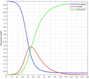
Figure 2: Dynamics of the SIR compartment model using the System Dynamics approach. Population SizeN= 1,000, con-tact rateβ = 15, infection probabilityγ =0.05, illness dura-tionδ = 15with initially 1 infected agent. Simulation run for 150 time-steps.
3
THE SIR MODEL
To explain the concepts of ABS and of our pure functional approach to it, we introduce the SIR model as a motivating example and use-case for our implementation. It is a very well studied and un-derstood compartment model from epidemiology [27] which allows to simulate the dynamics of an infectious disease like influenza, tuberculosis, chicken pox, rubella and measles spreading through a population [15].
In this model, people in a population of sizeNcan be in either one of three statesSusceptible,InfectedorRecoveredat a particular time, where it is assumed that initially there is at least one infected person in the population. People interact with each otheron aver-agewith a given rate ofβper time-unit and become infected with a given probabilityγ when interacting with an infected person. When infected, a person recoverson averageafterδ time-units and is then immune to further infections. An interaction between infected persons does not lead to re-infection, thus these interac-tions are ignored in this model. This definition gives rise to three compartments with the transitions seen in Figure 1.
This model was also formalized using System Dynamics (SD) [39]. In SD one models a system through differential equations, allowing to conveniently express continuous systems which change over time, solving them by numerically integrating over time which gives then rise to the dynamics. We won’t go into detail here and provide the dynamics of such a solution for reference purposes, shown in Figure 2.
An Agent-Based approach
The approach of mapping the SIR model to an ABS is to discretize the population and model each person in the population as an indi-vidual agent. The transitions between the states are happening due to discrete events caused both by interactions amongst the agents and time-outs. The major advantage of ABS is that it allows to incor-porate spatiality as shown in Section 4.3 and simulate heterogenity of population e.g. different sex, age. This is not possible with other simulation methods e.g. SD or Discrete Event Simulation [51].
According to the model, every agent makeson averagecontact withβrandom other agents per time unit. In ABS we can only contact discrete agents thus we model this by generating a random event on average everyβ1 time units. We need to sample from an exponential distribution because the rate is proportional to the size of the population [5]. Note that an agent does not know the other agents’ state when making contact with it, thus we need a mechanism in which agents reveal their state in which they are in
at the moment of making contact. This mechanism is an implemen-tation detail, which we will derive in our implemenimplemen-tation steps. For now we only assume that agents can make contact with each other somehow.
4
DERIVING A PURE FUNCTIONAL
APPROACH
We presented a high-level agent-based approach to the SIR model in the previous section, which focused only on the states and the transitions, but we haven’t talked about technical implementation. In [45] two fundamental problems of implementing an agent-based simulation from a programming-language agnostic point of view is discussed. The first problem is how agents can be pro-active and the second how interactions and communication be-tween agents can happen. For agents to be pro-active, they must be able to perceive the passing of time, which means there must be a concept of an agent-process which executes over time. Inter-actions between agents can be reduced to the problem of how an agent can expose information about its internal state which can be perceived by other agents. Further the authors have shown the influence of different deterministic and non-deterministic elements in agent-based simulation on the dynamics and how the influence of non-determinism can completely break them down or result in different dynamics despite same initial conditions. This means that we want to rule out any potential source of non-determinism.
In this section we will derive a pure functional approach for an agent-based simulation of the SIR model in which we will pose solutions to the previously mentioned problems. We will start out with a straight forward approach in Yampa and show its limitations. Then in further steps we will add more concepts and generalisations, ending up at the final approach which utilises Monadic Stream Functions, a generalisation of FRP.
Of paramount importance is to keep our implementations pure which rules out the use of the IO Monad and thus any potential source of non-determinism under all circumstances because we would loose all compile time guarantees about reproducibility. Still we will make use of the Random and State Monad which indeed
465 466 467 468 469 470 471 472 473 474 475 476 477 478 479 480 481 482 483 484 485 486 487 488 489 490 491 492 493 494 495 496 497 498 499 500 501 502 503 504 505 506 507 508 509 510 511 512 513 514 515 516 517 518 519 520 521 522
523 524
525 526
527 528
529 530 531
532 533
534 535
536 537 538
539 540
541 542
543 544
545 546 547
548 549
550 551
552 553 554
555 556
557 558
559 560
561 562 563
564 565
566 567
568 569
570 571 572
573 574
575 576
577 578 579
580 allow effects but the crucial point here is that we restrict
side-effects only to these types in a controlled way without allowing general unrestricted effects1.
4.1
Functional Reactive Programming
As described in the Section 2.2, Arrowized FRP [24] is a way to implement systems with continuous and discrete time-semantics where the central concept is the Signal Function, which can be understood as a process over time, mapping an input- to an output-signal. Technically speaking, a signal function is a continuation which allows to capture state using closures and hides away the∆t, which means that it is never exposed explicitly to the programmer, meaning it cannot be messed with.
The concept of processes over time is an ideal match for our agents and our system as a whole, thus we will implement them and the whole system as signal functions.
4.1.1 Implementation. We start by defining the SIR states as ADT and our agents as signal function (SF) which receives the SIR states of all agents as input and outputs the current SIR state of the agent:
dataSIRState=Susceptible| Infected|Recovered
typeSIRAgent=SF [SIRState] SIRState
Now we can define the behaviour of an agent to be the following: sirAgent::RandomGen g=> g-> SIRState-> SIRAgent
sirAgentgSusceptible=susceptibleAgent g sirAgentgInfected =infectedAgent g sirAgent_Recovered =recoveredAgent
Depending on the initial state we return the corresponding be-haviour. Note that we are passing a random-number generator instead of running in the Random Monad because signal functions as implemented in Yampa are not capable of being monadic.
We see that the recovered agent ignores the random-number generator because a recovered agent does nothing, stays immune forever and can not get infected again in this model. Thus a recov-ered agent is a consuming state from which there is no escape, it simply acts as a sink which returns constantlyRecovered: recoveredAgent:: SIRAgent
recoveredAgent= arr (constRecovered)
Lets look how we can implement the behaviour of a susceptible agent. It makes contacton averagewithβother random agents. For everyinfectedagent it gets into contact with, it becomes infected with a probability ofγ. If an infection happens, it makes the transi-tion to theInfectedstate. To make contact, it gets fed the states of all agents in the system from the previous time-step, so it can draw random contacts - this is one, very naive way of implementing the interactions between agents.
Thus a susceptible agent behaves as susceptible until it becomes infected. Upon infection anEvent is returned which results in switching into theinfectedAgentSF, which causes the agent to behave as an infected agent from that moment on. When an infec-tion event occurs we change the behaviour of an agent using the Yampa combinatorswitch, which is quite elegant and expressive as it makes the change of behaviour at the occurrence of an event
1The code of all steps can be accessed freely through the following URL: https://github.
com/thalerjonathan/phd/tree/master/public/purefunctionalepidemics/code
explicit. Note that to make contacton average, we use Yampas oc-casionallyfunction which requires us to carefully select the right ∆tfor sampling the system as will be shown in results.
susceptibleAgent:: RandomGeng=> g-> SIRAgent susceptibleAgentg=
switch (susceptible g) (const (infectedAgent g))
where
susceptible::RandomGen g
=> g-> SF [SIRState] (SIRState, Event())
susceptible g= proc as-> do
makeContact<- occasionally g (1 /contactRate)() -< ()
if isEvent makeContact
then(do
-- draw random element from the list
a <-drawRandomElemSF g -<as
casea of
Infected->do
-- returns True with given probability
i <-randomBoolSF g infectivity -<()
if i
thenreturnA-<(Infected, Event())
elsereturnA-<(Susceptible, NoEvent)
_ ->returnA-< (Susceptible,NoEvent))
elsereturnA-<(Susceptible, NoEvent)
To deal with randomness in an FRP way we implemented ad-ditional signal functions built on thenoiseRfunction provided by Yampa. This is an example for the stream character and statefulness of a signal function as it allows to keep track of the changed random-number generator internally through the use of continuations and closures. Here we provide the implementation ofrandomBoolSF.
drawRandomElemSF works similar but takes a list as input and returns a randomly chosen element from it:
randomBoolSF:: RandomGeng=> g ->Double -> SF() Bool randomBoolSFg p=proc_ -> do
r <- noiseR ((0,1):: (Double, Double)) g-< ()
returnA-< (r <=p)
An infected agent recoverson averageafterδtime units. This is implemented by drawing the duration from an exponential distri-bution [5] withλ=δ1 and making the transition to theRecovered
state after this duration. Thus the infected agent behaves as infected until it recovers, on average after the illness duration, after which it behaves as a recovered agent by switching intorecoveredAgent. As in the case of the susceptible agent, we use theoccasionally func-tion to generate the event when the agent recovers. Note that the infected agent ignores the states of the other agents as its behaviour is completely independent of them.
infectedAgent:: RandomGeng =>g ->SIRAgent
infectedAgentg =switch infected (const recoveredAgent)
where
infected:: SF[SIRState] (SIRState,Event ())
infected=proc _-> do
recEvt <- occasionally g illnessDuration()-< ()
leta =event Infected(constRecovered) recEvt
returnA-< (a, recEvt)
For running the simulation we use Yampas functionembed: runSimulation:: RandomGeng
=> g ->Time-> DTime-> [SIRState] ->[[SIRState]] runSimulationg t dt as
=embed (stepSimulation sfs as) ((), dts)
where
steps = floor (t/dt)
dts = replicate steps (dt,Nothing)
n = length as
(rngs,_)= rngSplits g n[] -- unique rngs for each agent
sfs = zipWith sirAgent rngs as
What we need to implement next is a closed feedbackloop -the heart of every agent-based simulation. Fortunately, [11, 31]
581 582 583 584 585 586 587 588 589 590 591 592 593 594 595 596 597 598 599 600 601 602 603 604 605 606 607 608 609 610 611 612 613 614 615 616 617 618 619 620 621 622 623 624 625 626 627 628 629 630 631 632 633 634 635 636 637 638
639 640
641 642
643 644
645 646 647
648 649
650 651
652 653 654
655 656
657 658
659 660
661 662 663
664 665
666 667
668 669 670
671 672
673 674
675 676
677 678 679
680 681
682 683
684 685
686 687 688
689 690
691 692
693 694 695
696 discusses implementing this in Yampa. The functionstepSimulation
is an implementation of such a closed feedback-loop. It takes the current signal functions and states of all agents, runs them all in parallel and returns this step’s new agent states. Note the use ofnotYetwhich is required because in Yampa switching occurs immediately att=0. If we don’t delay the switching att =0 until the next step, we would enter an infinite switching loop -notYet
simply delays the first switching until the next time-step. stepSimulation:: [SIRAgent]-> [SIRState] ->SF () [SIRState] stepSimulationsfs as =
dpSwitch
-- feeding the agent states to each SF
(\_sfs'-> (map (\sf -> (as, sf)) sfs')) -- the signal functions
sfs
-- switching event, ignored at t = 0
(switchingEvt>>>notYet)
-- recursively switch back into stepSimulation
stepSimulation
where
switchingEvt::SF ((), [SIRState]) (Event [SIRState])
switchingEvt=arr (\ (_, newAs)-> EventnewAs)
Yampa provides thedpSwitchcombinator for running signal functions in parallel, which has the following type-signature: dpSwitch::Functorcol
-- routing function
=>(forall sf.a ->col sf -> col (b, sf)) -- SF collection
->col (SFb c)
-- SF generating switching event ->SF (a, col c) (Eventd)
-- continuation to invoke upon event ->(col (SF b c)->d -> SFa (col c)) ->SF a (col c)
Its first argument is the pairing-function, which pairs up the input to the signal functions - it has to preserve the structure of the signal function collection. The second argument is the collection of signal functions to run. The third argument is a signal function generating the switching event. The last argument is a function, which generates the continuation after the switching event has occurred.dpSwitchreturns a new signal function, which runs all the signal functions in parallel and switches into the continuation when the switching event occurs. The d indpSwitchstands for decoupled which guarantees that it delays the switching until the next time-step: the function into which we switch is only applied in the next step, which prevents an infinite loop if we switch into a recursive continuation.
Conceptually,dpSwitchallows us to recursively switch back into thestepSimulationwith the continuations and new states of all the agents after they were run in parallel.
4.1.2 Results. The dynamics generated by this step can be seen in Figure 3.
By following the FRP approach we assume a continuous flow of time, which means that we need to select acorrect∆t otherwise we would end up with wrong dynamics. The selection of a correct ∆tdepends in our case onoccasionallyin thesusceptiblebehaviour, which randomly generates an event on average withcontact rate
following the exponential distribution. To arrive at the correct dynamics, this requires us to sampleoccasionally, and thus the whole system, with small enough∆twhich matches the frequency of events generated bycontact rate. If we choose a too large∆t, we loose events, which will result in wrong dynamics as can be seen in
(a)∆t=0.1 (b)∆t=0.01
Figure 3: FRP simulation of agent-based SIR showing the in-fluence of different∆t. Population size of 1,000 with contact rateβ = 15, infection probabilityγ = 0.05, illness duration
δ =15with initially 1 infected agent. Simulation run for 150 time-steps with respective∆t.
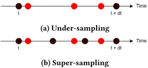
(a) Under-sampling
[image:6.612.324.556.84.197.2](b) Super-sampling
Figure 4: A visual explanation of under-sampling and super-sampling. The black dots represent the time-steps of the sim-ulation. The red dots represent virtual events which occur at specific points in continuous time. In the case of under-sampling, 3 events occur in between the two time steps but
occasionallyonly captures the first one. By increasing the sampling frequency either through a smaller∆t or super-sampling all 3 events can be captured.
Figure 3a. This issue is known as under-sampling and is described in Figure 4.
For tackling this issue we have two options. The first one is to use a smaller∆tas can be seen 3b, which results in the whole system being sampled more often, thus reducing performance. The other option is to implement super-sampling and apply it tooccasionally, which would allow us to run the whole simulation with∆t=1.0 and only sample theoccasionally function with a much higher frequency.
An approach to super-sampling would be to introduce a new combinator to Yampa which allows us to super-sample other signal functions.
superSampling:: Int->SF a b-> SFa [b]
It evaluates theSF argument forntimes, each with∆t = ∆nt and the same input argumentafor allnevaluations. At time 0 no super-sampling is performed and just a single output of the
SFargument is calculated. A list ofbis returned with length ofn
containing the result of thenevaluations of theSFargument. If 0 or less super samples are requested exactly one is calculated. We could then wrap the occasionally function which would then generate a
[image:6.612.362.512.287.356.2]697 698 699 700 701 702 703 704 705 706 707 708 709 710 711 712 713 714 715 716 717 718 719 720 721 722 723 724 725 726 727 728 729 730 731 732 733 734 735 736 737 738 739 740 741 742 743 744 745 746 747 748 749 750 751 752 753 754
755 756
757 758
759 760
761 762 763
764 765
766 767
768 769 770
771 772
773 774
775 776
777 778 779
780 781
782 783
784 785 786
787 788
789 790
791 792
793 794 795
796 797
798 799
800 801
802 803 804
805 806
807 808
809 810 811
812 list of events. We have investigated super-sampling more in-depth
but have to omit this due to lack of space.
4.1.3 Discussion. We can conclude that our first step already introduced most of the fundamental concepts of ABS:
•Time - the simulation occurs over virtual time which is mod-elled explicitly, divided intofixed∆t, where at each step all agents are executed.
•Agents - we implement each agent as an individual, with the behaviour depending on its state.
•Feedback - the output state of the agent in the current time-steptis the input state for the next time-stept+∆t.
•Environment - as environment we implicitly assume a fully-connected network (complete graph) where every agent ’knows’ every other agent, including itself and thus can make contact with all of them.
•Stochasticity - it is an inherently stochastic simulation, which is indicated by the random-number generator and the usage ofoccasionally,randomBoolSFanddrawRandomElemSF.
•Deterministic - repeated runs with the same initial random-number generator result in same dynamics. This may not come as a surprise but in Haskell we can guarantee that property statically already at compile time because our sim-ulation runsnotin the IO Monad. This guarantees that no external, uncontrollable sources of non-determinism can interfere with the simulation.
Using FRP in the instance of Yampa results in a clear, expressive and robust implementation. State is implicitly encoded, depending on which signal function is active. By using explicit time-semantics withoccasionallywe can achieve extremely fine grained stochastics by sampling the system with small∆t: we are treating it as a truly continuous time-driven agent-based system.
A very severe problem, hard to find with testing but detectable with in-depth validation analysis, is the fact that in thesusceptible
agent the same random-number generator is used inoccasionally,
drawRandomElemSFandrandomBoolSF. This means that all three stochastic functions, which should be independent from each other, are inherently correlated. This is something one wants to prevent under all circumstances in a simulation, as it can invalidate the dynamics on a very subtle level, and indeed we have tested the influence of the correlation in this example and it has an impact. We left this severe bug in for explanatory reasons, as it shows an example where functional programming actually encourages very subtle bugs if one is not careful. A possible solution would be to simply split the initial random-number generator insirAgentthree times (using one of the splited generators for the next split) and pass three random-number generators tosusceptible.
So far we have an acceptable implementation of an agent-based SIR approach. What we are lacking at the moment is a general treatment of an environment. To conveniently introduce it we want to make use of monads which is not possible using Yampa. In the next step we make the transition to Monadic Stream Functions as introduced in Dunai [37] which allows FRP within a monadic context.
4.2
Generalising to Monadic Stream Functions
A part of the library Dunai is BearRiver, a wrapper which re-implements Yampa on top of Dunai, which should allow us to easily replace Yampa with MSFs. This will enable us to run arbi-trary monadic computations in a signal function, which we will need in the next step when adding an environment.
4.2.1 Identity Monad.We start by making the transition to Bear-River by simply replacing Yampas signal function by BearBear-Rivers’ which is the same but takes an additional type parameterm, indi-cating the monadic context. If we replace this type-parameter with the Identity Monad, we should be able to keep the code exactly the same, except from a few type-declarations, because BearRiver re-implements all necessary functions we are using from Yampa. We simply re-define our agent signal function, introducing the monad stack our SIR implementation runs in:
typeSIRMonad =Identity
typeSIRAgent =SF SIRMonad[SIRState] SIRState
4.2.2 Random Monad.Using the Identity Monad does not gain us anything but it is a first step towards a more general solution. Our next step is to replace the Identity Monad by the Random Monad, which will allow us to get rid of the RandomGen arguments to our functions and run the whole simulation within the Random Monad with the full features of FRP. We start by re-defining the SIRMonad and SIRAgent:
typeSIRMonadg =Randg
typeSIRAgentg =SF (SIRMonadg) [SIRState]SIRState
The question is now how to access this Random Monad func-tionality within the MSF context. For the functionoccasionally, there exists a monadic pendantoccasionallyM which requires a MonadRandom type-class. Because we are now running within a MonadRandom instance we simply replaceoccasionallywith occa-sionallyM.
occasionallyM:: MonadRandomm=> Time-> b-> SFm a (Eventb)
4.2.3 Discussion.Running in the Random Monad within FRP is convenient but is not as compelling, as we could have achieved the same by passing RandomGen around as we already demonstrated. A benefit though is that it guarantees us that we won’t have correlated stochastics as discussed in the previous section. In the next step we introduce the concept of a read/write environment which we realise using a StateT monad. This will show the real benefit and gives a much more compelling example for the transition to MSFs.
4.3
Adding an environment
In this step we will add an environment in which the agents exist and through which they interact with each other. This is a funda-mentally different approach to agent interaction but is as valid as the approach in the previous steps.
In ABS agents are often situated within a discrete 2D environ-ment [17] which is simply a finiteNxMgrid with either a Moore or von Neumann neighbourhood (Figure 5). Agents are either static or can move freely around with cells allowing either single or multiple occupants.
We can directly map the SIR model to a discrete 2D environment by placing the agents on a corresponding 2D grid with an unre-stricted neighbourhood. The behaviour of the agents is the same but
813 814 815 816 817 818 819 820 821 822 823 824 825 826 827 828 829 830 831 832 833 834 835 836 837 838 839 840 841 842 843 844 845 846 847 848 849 850 851 852 853 854 855 856 857 858 859 860 861 862 863 864 865 866 867 868 869 870
871 872
873 874
875 876
877 878 879
880 881
882 883
884 885 886
887 888
889 890
891 892
893 894 895
896 897
898 899
900 901 902
903 904
905 906
907 908
909 910 911
912 913
914 915
916 917
918 919 920
921 922
923 924
925 926 927
928 (a) von Neumann (b) Moore
Figure 5: Common neighbourhoods in discrete 2D environ-ments of Agent-Based Simulation.
they select their interactions directly from the environment. Also instead of feeding back the states of all agents as inputs, agents now communicate through the environment by revealing their current state to their neighbours by placing it on their cell. Agents can read the states of all their neighbours which tells them if a neighbour is infected or not. For purposes of a more interesting approach, we restrict the neighbourhood to Moore (Figure 5b).
We also implemented this spatial approach in Java using the well known ABS library RePast [32], to have a comparison with a state of the art approach and came to the same results as shown in Figure 6. This supports that our pure functional approach can produce such results as well and compares positively to the state of the art in the ABS field.
4.3.1 Implementation.We start by defining our discrete 2D en-vironment for which we use an indexed two dimensional array. In each cell the agents will store their current state, thus we use the
SIRStateas type for our array data:
typeDisc2dCoord=(Int,Int)
typeSIREnv =Array Disc2dCoord SIRState
Next we redefine our monad stack and agent signal function. We use a StateT transformer on top of our Random Monad from the previous step withSIREnvas type for the state. Our agent signal function now has unit input and output type, which indicates that the actions of the agents are only visible through side-effects in the monad stack they are running in.
typeSIRMonadg= StateT SIREnv(Randg)
typeSIRAgentg= SF (SIRMonadg) () ()
The implementation of a susceptible agent is now a bit different. The agent directly queries the environment for its neighbours and randomly selects one of them. The remaining behaviour is similar: susceptibleAgent::RandomGen g=> Disc2dCoord->SIRAgentg susceptibleAgentcoord
=switch susceptible (const (infectedAgent coord))
where
susceptible:: RandomGeng
=> SF(SIRMonadg)() ((),Event ())
susceptible= proc_-> do
makeContact<- occasionallyM (1 /contactRate)() -<()
if not (isEvent makeContact)
thenreturnA-<((),NoEvent)
else(do
env<- arrM_ (lift get)-<()
letns =neighbours env coord agentGridSize moore
s<- drawRandomElemS -< ns
cases of
Infected ->do
infected<- arrM_
(lift $lift$ randomBoolM infectivity)-<()
if infected
then (do
arrM (put. changeCell coordInfected) -< env
returnA-< ((), Event()))
elsereturnA-<((),NoEvent)
_ ->returnA-< ((),NoEvent)) neighbours:: SIREnv ->Disc2dCoord-> Disc2dCoord
-> [Disc2dCoord]-> [SIRState] moore:: [Disc2dCoord]
moore= [ topLeftDelta, topDelta, topRightDelta,
leftDelta, rightDelta,
bottomLeftDelta, bottomDelta, bottomRightDelta ]
topLeftDelta:: Disc2dCoord topLeftDelta = (-1, -1) topDelta:: Disc2dCoord topDelta = (0, -1) ...
Querying the neighbourhood is done using theneighboursfunction. It takes the environment, the coordinate for which to query the neighbours for, the dimensions of the 2D grid and the neighbour-hood information and returns the data of all neighbours it could find. Note that on the edge of the environment, it could be the case that fewer neighbours than provided in the neighbourhood information will be found due to clipping.
The behaviour of an infected agent is similar to in the previous step, with the difference that upon recovery the infected agent updates its state in the environment from Infected to Recovered.
For running the simulation with MSFs we use the function em-bedwhich is not provided by BearRiver but by Dunai which has important implications. As already explained in the background Section 2.4, Dunai does not know about time in MSFs, which is what BearRiver builds on top of MSFs. Thus, when running our simulation usingembedwe get theReaderTin addition to the other Monad Transformers, which we need to run usingrunReaderT. Note that instead of returning agent states we simply return a list of envi-ronments, one for each step. The agent states can then be extracted from each environment.
runSimulation:: RandomGeng =>g ->Time ->DTime -> SIREnv ->[(Disc2dCoord, SIRState)]-> [SIREnv] runSimulationg t dt env as= evalRand esRand g
where
steps =floor (t/ dt)
dts =replicate steps ()
-- initial SFs of all agents
sfs =map (uncurry sirAgent) as
-- running the simulation
esReader=embed (stepSimulation sfs) dts
esState =runReaderT esReader dt
esRand =evalStateT esState env
Due to the different approach of returning the SIREnv in every step, we implemented our own MSF:
stepSimulation:: RandomGeng
=> [SIRAgentg] -> SF(SIRMonadg)() SIREnv stepSimulationsfs= MSF(\_ ->do
-- running all SFs with unit input
res<- mapM (`unMSF`()) sfs
-- extracting continuations, ignore output
letsfs'= fmap snd res
-- getting environment of current step
env<- get
-- recursive continuation
letct =stepSimulation sfs'
return (env, ct))
4.3.2 Results. We implemented rendering of the environments using the gloss library which allows us to cycle arbitrarily through
929 930 931 932 933 934 935 936 937 938 939 940 941 942 943 944 945 946 947 948 949 950 951 952 953 954 955 956 957 958 959 960 961 962 963 964 965 966 967 968 969 970 971 972 973 974 975 976 977 978 979 980 981 982 983 984 985 986
987 988
989 990
991 992
993 994 995
996 997
998 999
1000 1001 1002
1003 1004
1005 1006
1007 1008
1009 1010 1011
1012 1013
1014 1015
1016 1017 1018
1019 1020
1021 1022
1023 1024
1025 1026 1027
1028 1029
1030 1031
1032 1033
1034 1035 1036
1037 1038
1039 1040
1041 1042 1043
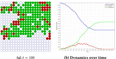
[image:9.612.60.290.83.200.2]1044 (a)t=100 (b) Dynamics over time
Figure 6: Simulating the agent-based SIR model on a 21x21 2D grid with Moore neighbourhood (Figure 5b), a single in-fected agent at the center and same SIR parameters as in Figure 2. Simulation run untilt = 200with fixed∆t = 0.1. Last infected agent recovers shortly aftert =160. The sus-ceptible agents are rendered as blue hollow circles for better contrast.
the steps and inspect the spreading of the disease over time visually as seen in Figure 6.
Note that the dynamics of the spatial SIR simulation which are seen in Figure 6b look quite different from the reference dynamics of Figure 2. This is due to a much more restricted neighbourhood which results in far fewer infected agents at a time and a lower number of recovered agents at the end of the epidemic, meaning that fewer agents got infected overall.
4.3.3 Discussion.At first the environment approach might seem a bit overcomplicated and one might ask what we have gained by using an unrestricted neighbourhood where all agents can contact all others. The real advantage is that we can introduce arbitrary restrictions on the neighbourhood as shown with the Moore neigh-bourhood.
Of course an environment is not restricted to be a discrete 2D grid and can be anything from a continuous N-dimensional space to a complex network - one only needs to change the type of the StateT monad and provide corresponding neighbourhood querying functions. The ability to place the heterogeneous agents in a generic environment is also the fundamental advantage of an agent-based over other simulation approaches and allows us to simulate much more realistic scenarios.
4.4
Additional Steps
ABS involves a few more advanced concepts which we don’t fully explore in this paper due to lack of space. Instead we give a short overview and discuss them without presenting code or going into technical details.
4.4.1 Agent-Transactions. Agent-transactions are necessary when an arbitrary number of interactions between two agents need to happen instantaneously without time-lag. The use-case for this are price negotiations between multiple agents where each pair of agents needs to come to an agreement in the same time-step [17].
In object-oriented programming, the concept of synchronous com-munication between agents is implemented directly with method calls.
We have implemented synchronous interactions, which we termed agent-transactions in an additional step. We solved it pure function-ally by running the signal functions of the transacting agent pair as often as their protocol requires but with∆t=0, which indicates the instantaneous character of agent-transactions.
4.4.2 Event Scheduling.Our approach is inherently time-driven where the system is sampled with fixed∆t. The other fundamental way to implement an ABS in general, is to follow an event-driven approach [30], which is based on the theory of Discrete Event Simulation [51]. In such an approach the system is not sampled in fixed∆tbut advanced as events occur where the system stays constant in between. Depending on the model, in an event-driven approach it may be more natural to express the requirements of the model.
In an additional step we have implemented a rudimentary event-driven approach, which allows the scheduling of events but had to omit it due to lack of space. Using the flexibility of MSFs we added a State transformer to the monad stack, which allows queuing of events into a priority queue. The simulation is advanced by process-ing the next event at the top of the queue, which means runnprocess-ing the MSF of the agent which receives the event. The simulation terminates if there are either no more events in the queue or after a given number of events, or if the simulation time has advanced to some limit. Having made the transition to MSFs, implementing this feature was quite straight forward, which shows the power and strength of the generalised approach to FRP using MSFs.
4.4.3 Dynamic Agent creation.In the SIR model, the agent pop-ulation stays constant - agents don’t die and no agents are created during simulation - but some simulations [17] require dynamic agent creation and destruction. We can easily add and remove agents signal functions in the recursive switch after each time-step. The only problem is that creating new agents requires unique agent ids but with the transition to MSFs we can add a monadic context, which allows agents to draw the next unique agent id when they create a new agent.
5
RELATED WORK
The amount of research on using pure functional programming with Haskell in the field of ABS has been moderate so far. Most of the papers are related to the field of Multi Agent Systems and look into how agents can be specified using the belief-desire-intention paradigm [13, 26, 44].
The author of [4] investigated in his master thesis Haskells paral-lel and concurrency features to implement (amongst others)HLogo, a Haskell clone of the ABS simulation package NetLogo, where agents run within the IO Monad and make use of Software Trans-actional Memory for a limited form of agent-interactions.
A library for DES and SD in Haskell calledAivika 3is described in the technical report [43]. It is not pure, as it uses the IO Monad under the hood and comes only with very basic features for event-driven ABS, which allows to specify simple state-based agents with timed transitions.
1045 1046 1047 1048 1049 1050 1051 1052 1053 1054 1055 1056 1057 1058 1059 1060 1061 1062 1063 1064 1065 1066 1067 1068 1069 1070 1071 1072 1073 1074 1075 1076 1077 1078 1079 1080 1081 1082 1083 1084 1085 1086 1087 1088 1089 1090 1091 1092 1093 1094 1095 1096 1097 1098 1099 1100 1101 1102
1103 1104
1105 1106
1107 1108
1109 1110 1111
1112 1113
1114 1115
1116 1117 1118
1119 1120
1121 1122
1123 1124
1125 1126 1127
1128 1129
1130 1131
1132 1133 1134
1135 1136
1137 1138
1139 1140
1141 1142 1143
1144 1145
1146 1147
1148 1149
1150 1151 1152
1153 1154
1155 1156
1157 1158 1159
1160 Using functional programming for DES was discussed in [26]
where the authors explicitly mention the paradigm of FRP to be very suitable to DES.
A domain-specific language for developing functional reactive agent-based simulations was presented in [48]. This language called FRABJOUS is human readable and easily understandable by domain-experts. It is not directly implemented in FRP/Haskell but is com-piled to Yampa code which they claim is also readable. This supports that FRP is a suitable approach to implement ABS in Haskell. Unfor-tunately, the authors do not discuss their mapping of ABS to FRP on a technical level, which would be of most interest to functional programmers.
Object-oriented programming and simulation have a long history together as the former one emereged out of Simula 67 [12] which was created for simulation purposes. Simula 67 already supported Discrete Event Simulation and was highly influential for today’s object-oriented languages. Although the language was important and influential, in our research we look into different approaches, orthogonal to the existing object-oriented concepts.
Lustre is a formally defined, declarative and synchronous dataflow programming language for programming reactive systems [19]. While it has solved some issues related to implementing ABS in Haskell it still lacks a few important features necessary for ABS. We don’t see any way of implementing an environment in Lustre as we do in our approach in Section 4.3. Also the language seems not to come with stochastic functions, which are but the very building blocks of ABS. Finally, Lustre does only support static networks, which is clearly a drawback in ABS in general where agents can be created and terminated dynamically during simulation.
There exists some research [14, 41, 47] of using the functional programming language Erlang [3] to implement ABS. The language is inspired by the actor model [1] and was created in 1986 by Joe Armstrong for Eriksson for developing distributed high reliability software in telecommunications. The actor model can be seen as quite influential to the development of the concept of agents in ABS which borrowed it from Multi Agent Systems [50]. It emphasises message-passing concurrency with share-nothing semantics, which maps nicely to functional programming concepts. The mentioned papers investigate how the actor model can be used to close the con-ceptual gap between agent-specifications, which focus on message-passing and their implementation. Further they also showed that using this kind of concurrency allows to overcome some problems of low level concurrent programming as well. Despite the natural mapping of ABS concepts to such an actor language it leads to simulations which despite same initial starting conditions might lead to different results due to concurrency.
6
CONCLUSIONS
Our FRP based approach is different from traditional approaches in the ABS community. First it builds on the already quite powerful FRP paradigm. Second, due to our continuous time approach, it forces one to think properly of time-semantics of the model and how small∆tshould be. Third it requires one to think about agent interactions in a new way instead of being just method-calls.
Because no part of the simulation runs in the IO Monad and we do not use unsafePerformIO we can rule out a serious class of bugs
caused by implicit data-dependencies and side-effects which can occur in traditional imperative implementations.
Also we can statically guarantee the reproducibility of the simu-lation, which means that repeated runs with the same initial con-ditions are guaranteed to result in the same dynamics. Although we allow side-effects within agents, we restrict them to only the Random and State Monad in a controlled, deterministic way and never use the IO Monad which guarantees the absence of non-deterministic side effects within the agents and other parts of the simulation.
Determinism is also ensured by fixing the∆tand not making it dependent on the performance of e.g. a rendering-loop or other system-dependent sources of non-determinism as described by [38]. Also by using FRP we gain all the benefits from it and can use research on testing, debugging and exploring FRP systems [35, 38].
Issues
Currently, the performance of the system is not comparable to imperative implementations. We compared the performance of our pure functional approach as presented in Section 4.3 to an implementation in Java using the ABS library RePast [32]. We ran the simulation untilt =100 on a 51x51 (2,601 agents) with∆t = 0.1 (unknown in RePast) and averaged 8 runs. The performance results make the lack of speed of our approach quite clear: the pure functional approach needs 100.3 seconds whereas the Java RePast version just 10.8 seconds on our machine to arrive att=100. We have already started investigating speeding up performance through the use of Software Transactional Memory [20, 21] which is quite straight forward when using MSFs. It shows very good results but we have to leave the investigation and optimization of the performance aspect of our approach for further research as it is out of the scope of this paper.
Despite the strengths and benefits we get by leveraging on FRP, there are errors that are not raised at compile time, e.g. we can still have infinite loops and run-time errors. This was for exam-ple investigated in [40] where the authors use dependent types to avoid some run-time errors in FRP. We suggest that one could go further and develop a domain specific type system for FRP that makes the FRP based ABS more predictable and that would sup-port further mathematical analysis of its properties. Furthermore, moving to dependent types would pose a unique benefit over the traditional object-oriented approach and should allow us to express and guarantee even more properties at compile time. We leave this for further research.
In our pure functional approach, agent identity is not as clear as in traditional object-oriented programming, where an agent can be hidden behind a polymorphic interface which is much more abstract than in our approach. Also the identity of an agent is much clearer in object-oriented programming due to the concept of object-identity and the encapsulation of data and methods.
We can conclude that the main difficulty of a pure functional approach evolves around the communication and interaction be-tween agents, which is a direct consequence of the issue with agent identity. Agent interaction is straight-forward in object-oriented programming, where it is achieved using method-calls mutating the internal state of the agent, but that comes at the cost of a new class
1161 1162 1163 1164 1165 1166 1167 1168 1169 1170 1171 1172 1173 1174 1175 1176 1177 1178 1179 1180 1181 1182 1183 1184 1185 1186 1187 1188 1189 1190 1191 1192 1193 1194 1195 1196 1197 1198 1199 1200 1201 1202 1203 1204 1205 1206 1207 1208 1209 1210 1211 1212 1213 1214 1215 1216 1217 1218
1219 1220
1221 1222
1223 1224
1225 1226 1227
1228 1229
1230 1231
1232 1233 1234
1235 1236
1237 1238
1239 1240
1241 1242 1243
1244 1245
1246 1247
1248 1249 1250
1251 1252
1253 1254
1255 1256
1257 1258 1259
1260 1261
1262 1263
1264 1265
1266 1267 1268
1269 1270
1271 1272
1273 1274 1275
1276 of bugs due to implicit data flow. In pure functional programming
these data flows are explicit but our current approach of feeding back the states of all agents as inputs is not very general. We have added further mechanisms of agent interaction which we had to omit due to lack of space.
7
FURTHER RESEARCH
We see this paper as an intermediary and necessary step towards dependent types for which we first needed to understand the po-tential and limitations of a non-dependently typed pure functional approach in Haskell. Dependent types are extremely promising in functional programming as they allow us to express stronger guar-antees about the correctness of programs and go as far as allowing to formulate programs and types as constructive proofs which must be total by definition [2, 29, 46].
So far no research using dependent types in agent-based simu-lation exists at all. In our next paper we want to explore this for the first time and ask more specifically how we can add dependent types to our pure functional approach, which conceptual implica-tions this has for ABS and what we gain from doing so. We plan on using Idris [6] as the language of choice as it is very close to Haskell with focus on real-world application and running programs as opposed to other languages with dependent types e.g. Agda and Coq which serve primarily as proof assistants.
We hypothesize that dependent types could help ruling out even more classes of bugs at compile time and encode invariants and model specifications on the type level, which implies that we don’t need to test them using e.g. property-testing with QuickCheck. This would allow the ABS community to reason about a model directly in code. We think that a promising approach is to follow the work of [7–10, 18] in which the authors utilize GADTs to implement an indexed monad which allows to implementation correct-by-construction software.
•Accessing the environment in section 4.3 involves indexed array access which is always potentially dangerous as the indices have to be checked at run-time.
Using dependent types it should be possible to encode the environment dimensions into the types. In combination with suitable data types for coordinates one should be able to ensure already at compile time that access happens only within the bounds of the environment.
•In the SIR implementation one could make wrong state-transitions e.g. when an infected agent should recover, noth-ing prevents one from maknoth-ing the transition back to suscep-tible.
Using dependent types it might be possible to encode invari-ants and state-machines on the type level which can prevent such invalid transitions already at compile time. This would be a huge benefit for ABS because many agent-based models define their agents in terms of state-machines.
•An infected agent recovers after a given time - the transi-tion of infected to recovered is a timed transitransi-tion. Nothing prevents us fromneverdoing the transition at all.
With dependent types we might be able to encode the passing of time in the types and guarantee on a type level that an
infected agent has to recover after a finite number of time steps.
• In more sophisticated models agents interact in more com-plex ways with each other e.g. through message exchange using agent IDs to identify target agents. The existence of an agent is not guaranteed and depends on the simulation time because agents can be created or terminated at any point during simulation.
Dependent types could be used to implement agent IDs as a proof that an agent with the given id existsat the current time-step. This also implies that such a proof cannot be used in the future, which is prevented by the type system as it is not safe to assume that the agent will still exist in the next step.
• In our implementation, we terminate the SIR model always after a fixed number of time-steps. We can informally reason that restricting the simulation to a fixed number of time-steps is not necessary because the SIR modelhas toreach a steady state after a finite number of steps. This means that at that point the dynamics won’t change any more, thus one can safely terminate the simulation. Informally speaking, the reason for that is that eventually the system will run out of infected agents, which are the drivers of the dynamic. We know that all infected agents will recover after a finite number of time-stepsandthat there is only a finite source for infected agents which is monotonously decreasing. Using dependent types it might be possible to encode this in the types, resulting in a total simulation, creating a corre-spondence between the equilibrium of a simulation and the totality of its implementation. Of course this is only possible for models in which we know about their equilibria a priori or in which we can reason somehow that an equilibrium exists.
ACKNOWLEDGMENTS
The authors would like to thank I. Perez, H. Nilsson, J. Greensmith, M. Baerenz, H. Vollbrecht, S. Venkatesan and J. Hey for constructive feedback, comments and valuable discussions.
REFERENCES
[1] Gul Agha. 1986.Actors: A Model of Concurrent Computation in Distributed Systems. MIT Press, Cambridge, MA, USA.
[2] Thorsten Altenkirch, Nils Anders Danielsson, Andres Loeh, and Nicolas Oury. 2010. Pi Sigma: Dependent Types Without the Sugar. InProceedings of the 10th In-ternational Conference on Functional and Logic Programming (FLOPS’10). Springer-Verlag, Berlin, Heidelberg, 40–55. https://doi.org/10.1007/978-3-642-12251-4_5 [3] Joe Armstrong. 2010. Erlang.Commun. ACM53, 9 (Sept. 2010), 68–75. https:
//doi.org/10.1145/1810891.1810910
[4] Nikolaos Bezirgiannis. 2013.Improving Performance of Simulation Software Using Haskells Concurrency & Parallelism. Ph.D. Dissertation. Utrecht University - Dept. of Information and Computing Sciences.
[5] Andrei Borshchev and Alexei Filippov. 2004. From System Dynamics and Discrete Event to Practical Agent Based Modeling: Reasons, Techniques, Tools. Oxford. [6] Edwin Brady. 2013. Idris, a general-purpose dependently typed programming
language: Design and implementation.Journal of Functional Programming23, 05 (2013), 552–593. https://doi.org/10.1017/S095679681300018X
[7] Edwin Brady. 2013. Programming and Reasoning with Algebraic Effects and Dependent Types. InProceedings of the 18th ACM SIGPLAN International Confer-ence on Functional Programming (ICFP ’13). ACM, New York, NY, USA, 133–144. https://doi.org/10.1145/2500365.2500581
[8] Edwin Brady. 2016. State Machines All The Way Down - An Architecture for Dependently Typed Applications. Technical Report. https://www.idris-lang.org/