Smooth and sharp creation of a pointlike source
for a (3 + 1)-dimensional quantum field
L. J. Zhou,1,2,3,4,* Margaret E. Carrington,1,2,† Gabor Kunstatter,2,3,‡ and Jorma Louko5,§ 1Department of Physics, Brandon University, Brandon, Manitoba, R7A 6A9 Canada
2
Winnipeg Institute for Theoretical Physics, Winnipeg, Manitoba
3Department of Physics, University of Winnipeg, Winnipeg, Manitoba, R3B 2E9 Canada 4
Department of Physics and Astronomy, University of Manitoba, Winnipeg, Manitoba, R3T 2N2 Canada 5School of Mathematical Sciences, University of Nottingham, Nottingham NG7 2RD, United Kingdom
(Received 6 January 2017; published 10 April 2017)
We analyze the smooth and sharp creation of a pointlike source for a quantized massless scalar field in (3þ1)-dimensional Minkowski spacetime, as a model for the breakdown of correlations that has been proposed to occur at the horizon of an evaporating black hole. The creation is implemented by a time-dependent self-adjointness parameter at the excised spatial origin. In a smooth creation, the renormalized energy densityhT00iis well defined away from the source, but it is unbounded both above and below: the outgoing pulse contains an infinite negative energy, while a cloud of infinite positive energy lingers near the fully-formed source. In the sharp creation limit,hT00idiverges everywhere in the timelike future of the creation event, and so does the response of an Unruh-DeWitt detector that operates in the timelike future of the creation event. The source creation is significantly more singular than the corresponding process in
1þ1dimensions, analyzed previously, and it may be sufficiently singular to break quantum correlations as proposed in a black hole spacetime.
DOI:10.1103/PhysRevD.95.085007
I. INTRODUCTION
In quantum field theory, it has been long known that a time dependent boundary condition or a time dependent metric can create particles and energy flows. Parker’s pioneering work showed that a Klein-Gordon field on an expanding cosmological spacetime undergoes particle cre-ation [1]. Moore showed that particle creation can be induced by varying the length of a cavity [2], while Candelas and Deutsch showed that even a single accel-erating mirror can induce a flux of particles and energy[3]; this phenomenon is now known as the Dynamical (or non-stationary) Casimir Effect, and it was observed in 2011 using a photon analogue system[4]. The most celebrated example is Hawking’s prediction of black hole radiation [5], whose observation in analogue quantum systems may be at the threshold of current technology [6,7].
In order to reconcile the thermal character of Hawking radiation with fundamental unitarity of quantum theory, it has been proposed[8–14] that the horizon of a radiating black hole could be more singular than the conventional picture of quantum fields on the classical black hole spacetime suggests [15–17]. While detailed modeling of this possible singularity remains elusive, the key proposed feature is that the singularity should break down
correlations between the two sides of the horizon. A context in which such breaking of correlations can be studied is quantum field theory on a fixed background spacetime. One way to do this is to write down by hand a quantum state in which the correlations are absent[18,19]. Another is to allow an impermeable wall to develop where initially there was none[20–23]. The purpose of the present paper is to improve the understanding of the latter scenario. When the impermeable wall is inserted quickly, a surprising feature emerges: for a massless scalar field in 1þ1 dimensions, the energy transmitted into the field diverges in the limit of rapid wall creation, but the response of an Unruh-DeWitt detector [24,25] crossing this pulse of diverging energy remains finite[22]. The finite detector response casts doubt on the ability of wall creation, however rapid, to break down quantum correlations suffi-ciently strongly to save unitarity in an evolving black hole spacetime. One limitation of the analysis in[22]is however that it was done in 1þ1 dimensions. Quantum fields generally become more singular as the spacetime dimen-sion increases: would the concludimen-sions in3þ1dimensions be similar? A second limitation is that the analysis in[22] relied on an infrared cutoff to eliminate the infrared ambiguity that the massless scalar field has in 1þ1 dimensions. Could the results in [22] be an artifact of the (1þ1)-dimensional infrared sickness, with no counter-part in3þ1dimensions?
In this paper we take a first step toward adapting the wall creation analysis of[22]to3þ1dimensions, and answer-ing these questions. We consider a massless scalar field in *[email protected]
(3þ1)-dimensional Minkowski spacetime, and we intro-duce at the spatial origin a time-dependent boundary condition that interpolates, over a finite interval of time, between ordinary Minkowski dynamics and a Dirichlet-type condition. As the boundary condition is introduced at just one spatial point, the physical interpretation is now not the smooth creation of a wall but the smooth creation of a pointlike source. We then ask what happens to the energy transmitted into the field and to the response of an Unruh-DeWitt detector in the limit of rapid source creation. The answers turn out to have some similarities with the (1þ1)-dimensional analysis of [22] but also significant differences. A technical difference is that in 3þ1 dimen-sions there is no infrared ambiguity, and no infrared cutoff is needed. A difference in physically observable quantities is that in3þ1dimensions both the field’s energy density and the detector’s response are more singular.
First, we consider the energy. While the renormalized energy densityhT00iis well defined everywhere away from the source, it is bounded neither above nor below. In the outgoing pulse generated by the evolving source,hT00iis unbounded below immediately to the future of the light cone of the point where the boundary condition starts to change, and the total energy in the pulse is negative infinity. After the pulse has gone,hT00iis nonzero, and it diverges at r→0 proportionally to −ðlnrÞ=r4: a cloud of positive energy lingers near the source after the source is fully formed, and the total energy in this cloud is positive infinity. Further, at a fixed r, hT00i is not static, and it diverges at t→∞ proportionally to lnt. In the limit of rapid source creation, hT00i diverges everywhere in the timelike future of the creation event. The source creation hence leaves in the late time region a large energetic memory. This memory has no counterpart in the (1þ1 )-dimensional analysis of [22].
We note that the firewall in both the previous paper[22] and the present work is not in fact modeled by the wall or point source, respectively, where the boundary conditions are specified. Instead, these serve as the source of the firewall which itself is modelled by the resulting outgoing null shell of energy. It is for this reason that it is important to calculate the response of a detector passing through the outgoing shell of energy (i.e. firewall), as we do in Sec.IV. In particular, we consider the response of a static Unruh-DeWitt detector. We find that the response of a detector that operates only in the late time region mimics hT00i closely, both in the late time limit and in the limit of rapid source creation: in both limits, the response has a logarithmic divergence. We have not considered in detail the response of a detector that goes through the pulse emanating from the changing boundary condition, but the behavior in the post-pulse region is already sufficient to establish that the response does not remain finite in the limit of rapid source creation.
We conclude that the rapid creation of a source makes the (3þ1)-dimensional field significantly more singular than
the corresponding event in1þ1dimensions; in particular, the response of an Unruh-DeWitt detector diverges in the rapid creation limit. These results suggest that a source creation may be able to model the breaking of quantum correlations in the way that has been proposed to happen in an evolving black hole spacetime[8–14]. The persistence of large late time effects is perhaps particularly reminiscent of the energetic curtain scenario proposed in[8].
We begin in Sec.IIby setting up the classical dynamics of the scalar field under the evolving boundary condition at the spatial origin. SectionIIIintroduces the quantized field and evaluates hT00i. The response of an Unruh-DeWitt detector is considered in Sec.IV. Section V gives a brief summary and discussion. Technical material is relegated to five appendices.
Our metric signature is mostly minus. Overline denotes complex conjugation. A continuous function of a real variable is said to be C0, a function that is n∈N¼ f1;2;…g times continuously differentiable is said to be Cn, and a function that has all derivatives is said to beC∞, or smooth. We work in geometric units in which ℏ¼c¼1.
II. CLASSICAL FIELD
A. Field equation and boundary condition
We consider a real massless scalar field ϕ in (3þ1 )-dimensional Minkowski spacetime from which the spatial origin has been excised. Writing the metric as
ds2¼dt2−ðdx1Þ2−ðdx2Þ2−ðdx3Þ2; ð2:1Þ
the field equation is
ð∂2
t −∇2Þϕ¼0; ð2:2Þ
where∇2¼∂2x1þ∂2x2þ∂2x3. The Klein-Gordon inner
prod-uct evaluated on a constantthypersurface reads
ðϕ1;ϕ2ÞKG¼i Z
dx1dx2dx3ðϕ1∂tϕ2−ð∂tϕ1Þϕ2Þ: ð2:3Þ
In the spherical coordinates, defined by ðx1; x2; x3Þ ¼ ðrsinθcosφ; rsinθsinφ; rcosθÞ, the metric reads
ds2¼dt2−dr2−r2ðdθ2þsin2θdφ2Þ ð2:4Þ
and the Klein-Gordon inner product reads
ðϕ1;ϕ2ÞKG¼i
Z ∞
0 r
2dr
Z
S2
dΩðϕ1∂tϕ2−ð∂tϕ1Þϕ2Þ;
ð2:5Þ
wheredΩ¼sinθdθdφis the volume element on unitS2. The excised spatial origin is atr¼0.
To specify the dynamics, we need to define∇2 at each t as a self-adjoint operator. After decomposition into spherical harmonics, the only freedom is in the spherically symmetric sector, as discussed in Appendix A: writing
ϕðt; rÞ ¼fðt; rffiffiffiffiffiffiÞ 4π p
r; ð2:6Þ
the eigenfunctions of ∇2 must satisfy the boundary condition
ðcosθðtÞÞlim
r→0fðt; rÞ ¼LðsinθðtÞÞlimr→0∂rfðt; rÞ; ð2:7Þ
where L is a positive constant of dimension length, introduced for dimensional convenience, and the prescribed functionθðtÞ, taking values in½0;πÞ, specifies at eachtthe self-adjoint extension of ∇2. We denote this extension byΔθðtÞ.
Δ0 coincides with the unique self-adjoint extension of
∇2onL
2ðR3Þ, yielding usual scalar field dynamics on full
Minkowski space. For θ∈ðπ=2;πÞ, Δθ has a positive proper eigenvalue, which on quantization would give a tachyonic instability. We therefore assumeθ∈½0;π=2, in which case the spectrum of Δθ consists of the negative continuum.
We specialize to aθðtÞ that interpolates betweenθ¼0 and θ¼π=2 over a finite interval of time. We may parametrize θðtÞas
θðtÞ ¼
8 < :
0 for t≤0; arccot½λLcotðhðλtÞÞ for 0< t <λ−1;
π=2 for t≥λ−1;
ð2:8Þ
whereλis a positive constant of dimension inverse length andh∶R→R is a smooth function such that
hðyÞ ¼0 fory≤0; ð2:9aÞ
0< hðyÞ<π=2 for 0< y <1; ð2:9bÞ
hðyÞ ¼π=2 for y≥1: ð2:9cÞ
Over the interval0< t <λ−1, the boundary condition(2.7) then reads
lim r→0
∂rfðt; rÞ
fðt; rÞ ¼λcotðhðλtÞÞ: ð2:10Þ
In words, this parametrization means that the boundary condition interpolation takes place over timeλ−1while the interpolation profile is determined by the dimensionless function hðyÞ. The limit of rapid interpolation with fixed profile is that of λ→∞.
B. Mode functions
As preparation for quantization, we shall write down the mode solutions that reduce to the usual Minkowski modes fort≤0. As noted above, we need consider only the spherically symmetric sector.
We work in the radial null coordinates u≔t−r and v≔tþr, in whicht¼ ðvþuÞ=2andr¼ ðv−uÞ=2. The metric (2.4)becomes
ds2¼dudv−1
4ðv−uÞ2ðdθ2þsin2θdφ2Þ: ð2:11Þ
Taking ϕ to be spherically symmetric, the field equa-tion(2.2) becomes
∂u∂vðrϕÞ ¼0: ð2:12Þ
We hence seek mode solutions with the ansatz
ϕk ¼ Uffiffiffiffiffiffik
4π p
r; ð2:13Þ
where
Ukðu; vÞ ¼ 1
ffiffiffiffiffiffiffiffi
4πk
p ½e−ikvþEkðuÞ; ð2:14Þ
k >0, andEkis to be found. As any choice forEksatisfies the wave equation, the task is to determineEk so that the boundary condition(2.7)is satisfied for alltand the usual Minkowski modes are obtained fort≤0.
Substituting(2.14)in the boundary condition(2.7)gives forEk the ordinary differential equation
LsinðθðtÞÞd dt½e
−ikt−EkðtÞ ¼cosðθðtÞÞ½e−iktþEkðtÞ:
ð2:15Þ
Writing
EkðuÞ ¼Rk=λðλuÞ ð2:16Þ
and using(2.8),(2.15)takes the dimensionless form
sinðhðyÞÞ d dy½e
−iKy−R
KðyÞ ¼cosðhðyÞÞ½e−iKyþRKðyÞ; ð2:17Þ
where K¼k=λ>0 is the dimensionless frequency and y¼λu.
To solve(2.17), we introduce the auxiliary function
BðyÞ ¼
8 < :
0 fory≤0; expð−R1
ycotðhðzÞÞdzÞ for0< y <1; 1 fory≥1:
BðyÞ is everywhere smooth: smoothness aty¼1follows from the smoothness ofhðzÞnearz¼1, and smoothness at y¼0is shown in Appendix B. For y >0, BðyÞsatisfies
B0ðyÞ
BðyÞ ¼cotðhðyÞÞ: ð2:19Þ
It follows that the solution to(2.17) is
RKðyÞ ¼
−e−iKy fory≤0;
−e−iKy−2iK BðyÞ
Ry
0BðzÞe−iKzdz for0< y <∞:
ð2:20Þ
From(2.20)and the smoothness ofBwe see thatRKðyÞis smooth everywhere except possibly aty¼0, and we verify in AppendixBthatRKðyÞisC25aty¼0. It follows that the mode functions are smooth everywhere except possibly at r¼t, and they are at leastC25 atr¼t.
An alternative expression forRKðyÞ is
RKðyÞ ¼
8 > > < > > :
−e−iKy for y≤0; e−iKy− 2
BðyÞ
Ry
0B0ðzÞe−iKzdz for 0< y <1;
e−iKy−2CK for y≥1; ð2:21Þ
where
CK¼
Z 1
0 B
0ðzÞe−iKzdz: ð2:22Þ
Atu≤0andu≥λ−1, the mode functionsϕk(2.13)hence reduce respectively to
ϕkðt; rÞ ¼
8 < :
−ie−iktsinðkrÞ
2πpffiffikr foru≤0; e−iktcosðkrÞ−C
k=λ
2πpffiffikr foru≥λ
−1: ð2:23Þ
For u≤0, ϕkðt; rÞ coincide with the usual Minkowski space mode functions. Evaluating the Klein-Gordon inner product (2.5) on a hypersurface of constant negative t shows that the normalization is ðϕk;ϕk0ÞKG¼δðk−k0Þ. Foru≥λ−1, ther-dependence in the numerator ofϕkðt; rÞ (2.23)contains the term cosðkrÞ, which one would expect from the boundary condition (2.7) with θ¼π=2, but it contains also the additive memory term −Ck=λ, which carries a recollection of how the boundary condition evolved from θ¼0to θ¼π=2. From (2.22)we see that CK is smooth inK,C0¼1, and CK→0 faster than any inverse power of K as K→∞, as can be verified by repeated integration by parts[26]. For fixedλ, the memory term is hence insignificant at large frequencies but
significant at low frequencies. We shall see in Sec.IIIthat the memory term has a significant effect on the stress-energy tensor and the Wightman function.
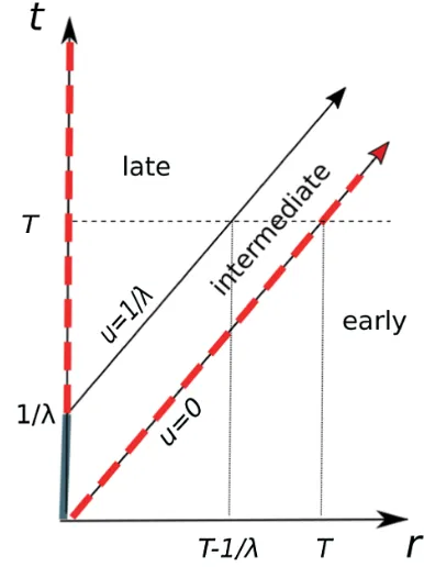
A spacetime diagram is shown in Fig. 1, indicating the regionsu <0,0< u <λ−1 andu >λ−1.
III. QUANTIZED FIELD A. Field operator and the Fock vacuum
We quantize the field by using for the spherically symmetric sector the mode functions found in Sec. II and treating the nonzero angular momentum sectors as in ordinary Minkowski space. As we are interested in the effects due to the evolving boundary condition, compared with a field in ordinary Minkowski space, we write out only the expressions for the spherically symmetric sector.
[image:4.612.337.530.46.304.2]We expand the spherically symmetric sector of the quantized field as
FIG. 1. Spacetime diagram of the evolving boundary condition
(2.7) at r¼0, with the angular dimensions suppressed. The interpolation betweenθ¼0 and θ¼π=2atr¼0occurs over
0< t <λ−1(solid line), and the null cones of the events where the boundary condition changes fill the region0< u <λ−1in the spacetime. The early region u <0 is outside the null cone of
ðt; rÞ ¼ ð0;0Þ, and the mode functions there coincide with those in full Minkowski space. The mode functions in the late region u >λ−1carry a memory of the field evolution that occurred over the intermediate region0< u <λ−1. The infinite contributions to the energy atr¼0(positive infinity) andr¼t(negative infinity) are shown as heavy dashed lines. The spacelike hypersurface t¼T >λ−1, shown as a short dashed line, intersects all three regions.
ϕ¼
Z ∞
0 ðakϕkþa
†
kϕkÞdk; ð3:1Þ
where the annihilation and creation operators have the commutators½ak; a†k0 ¼δðk−k0Þ. By the normalization of
the mode functions, this gives the field and its time derivative the correct equal-time commutator. We denote byj0ithe state that is annihilated by allak and by all the annihilation operators of the nonzero angular momentum sectors. In the regionu <0, j0i coincides with the usual Minkowski vacuum, which we denote byj0Mi.
B. Energy density
In the Lorentz frame of the metric (2.4), the energy density of the classical scalar field is given in terms of the energy-momentum tensor by
T00¼TuuþTvvþ2Tuv; ð3:2Þ
where [15]
Tuu¼ ð∂uϕÞ2; ð3:3aÞ
Tvv ¼ ð∂vϕÞ2; ð3:3bÞ
Tuv¼Tvu¼ 1
4r2½ð∂θϕÞ
2þ ðsinθÞ−2ð∂
φϕÞ2; ð3:3cÞ
and we have taken the scalar field to be minimally coupled. To obtain the renormalized energy density of the quantized field in the state j0i, hT00i≔h0jT00j0iren, we point-split the expressions in(3.3), take the expectation value inj0i, renormalize by subtracting the corresponding expectation value inj0Mi, and finally take the coincidence limit. Asj0i andj0Midiffer only in the spherically symmetric sector, the derivatives in(3.3c)show thathTuvi ¼0, and we find
hT00i ¼ lim u1;u2→u v1;v2→v
ð∂u1∂u2þ∂v1∂v2Þ½h0jϕð1Þϕð2Þj0i
−h0Mjϕð1Þϕð2Þj0Mi; ð3:4Þ
whereϕnow stands for the spherically symmetric quantum field (3.1).
To evaluate(3.4), we writeϕin terms of f as in (2.6). Recalling that r¼ ðv−uÞ=2, this gives
hT00i ¼ 1 4π
hð
∂ufÞ2i r2 þ
hð∂vfÞ2i r2
þhfð∂uf−∂vfÞi þ hð∂uf−∂vfÞfi 2r3 þ
hf2i 2r4
:
ð3:5Þ
By (2.6),(2.13)and(3.1), f has the expansion
f¼
Z ∞
0 ðakUkþa
†
kUkÞdk: ð3:6Þ
From(2.14),(2.16)and(3.6)we obtain forhT00ithe final expression
hT00i ¼ λ
2
16π2r2
Z ∞
0
dK K ½jR
0
Kðλðt−rÞÞj2−K2
− 1 32π2r2
∂ ∂r
Gλðt; rÞ
r
; ð3:7Þ
where the prime onRKdenotes the derivative with respect to the argument and
Gλðt; rÞ ¼
Z ∞
0
dK K
jRKðλðt−rÞÞj2þ2cosð2KλrÞ−1
þRKðλðt−rÞÞeiKλðtþrÞþR
Kðλðt−rÞÞe−iKλðtþrÞ
:
ð3:8Þ
The first term in(3.7)comes from the first term in(3.5), the second term in(3.7)comes from the last two terms in (3.5), and the second term in (3.5) vanishes. We note in passing that Gλ is related to the renormalized vacuum polarizationhϕ2i by
hϕ2i ¼Gλðt; rÞ
16π2r2: ð3:9Þ
C. Energy density in the early, late and intermediate regions
We considerhT00iseparately in the early region, t < r, in the late region, t > rþλ−1, and in the intermediate region,r≤t≤rþλ−1.
In the early region,t < r,j0i coincides withj0Mi, and hT00i vanishes. This can be seen immediately from(3.4), and also by substituting(2.20)into (3.7)and(3.8).
In the late region, t > rþλ−1, the first term in (3.7) vanishes. We show in AppendixCthathT00iis a pointwise well defined function, it has dependence on bothtandr, it is continuous, and it has the asymptotic forms
hT00i∼ lnt
4π2r4 ast→∞ with rfixed; ð3:10aÞ
hT00i∼ − lnr
8π2r4 asr→0 with t fixed: ð3:10bÞ
hence an infinite total energy, due to positive hT00i that diverges asr→0.
In the intermediate region,r≤t≤rþλ−1, we show in AppendixDthathT00iis a pointwise well-defined function, and it is continuous in r for t > r. Under the technical assumption that the third derivative of tanðhðyÞÞ is non-negative for sufficiently small positive y, we show in addition thathT00i is well defined also att¼r(where it then vanishes); however, due to contributions from the first term in (3.7), hT00i tends to negative infinity as r→t−, faster than any negative multiple of 1=hðλðt−rÞÞ. In particular, hT00i is not continuous at r¼t. This implies that integrating hT00i on a hypersurface of t¼T¼ constant>0 over an an arbitrarily small neighborhood of r¼T gives negative infinite energy. The changing boundary condition creates a pulse of infinite negative energy traveling outward, immediately to the future of the light cone of the point ðt; rÞ ¼ ð0;0Þ where the boundary condition starts to change.
Combining the results of the two previous paragraphs, it follows that the total energy on the hypersurface of t¼T¼constant withT >λ−1is not defined, even though hT00iexists at every point. Given anr0∈ð0; TÞ, the total energy forr≤r0is positive infinite, due to a large positive contribution fromr→0, while the total energy forr≥r0is negative infinite, due to a large negative contribution from r→T−.
D. Rapid boundary condition change
Finally, consider the limit in which the boundary con-dition changes rapidly,λ→∞. At each given point in the regiont > r,hT00idiverges in this limit, with the asymp-totic form
hT00i∼ lnλ
8π2r4; ð3:11Þ
as we show in Appendix C. In the limit of rapid source creation,hT00ihence diverges everywhere inside the light cone of the creation event. This is in a stark contrast to the corresponding (1þ1)-dimensional wall creation, where hT00i vanishes inside the light cone of the creation event [22].
IV. RESPONSE OF AN UNRUH-DEWITT DETECTOR
In this section we consider an inertial Unruh-DeWitt (UDW) detector[24,25]at a fixed spatial location.
We consider a detector that is coupled linearly to the quantum field. Within first-order perturbation theory, the probability of the detector to undergo a transition from a state with energy 0 to a state with energyωis proportional to the response function, given by[15,16,24,25]
FðωÞ ¼
Z ∞
−∞dt1
Z ∞
−∞dt2e
−iωðt1−t2Þχðt
1Þχðt2ÞWðt1; t2Þ;
ð4:1Þ
where the smooth real-valued switching functionχ spec-ifies how the detector’s interaction with the field is turned on and off, andW is the pull-back of the field’s Wightman function to the detector’s worldline. In the Minkowski vacuumj0Mi, we have [15]
Wj0Miðt1; t2Þ ¼−
1 4π2ðt
1−t2−iϵÞ2
; ð4:2Þ
where the limit ϵ→0þ is implied and encodes the
distributional part of W, and from (4.1) we obtain [18,27,28]
Fj0MiðωÞ ¼−
ωΘð−ωÞ 2π
Z ∞
−∞du½χðuÞ 2
þ 1
2π2
Z ∞
0 ds
cosðωsÞ s2
×
Z ∞
−∞duχðuÞ½χðuÞ−χðu−sÞ; ð4:3Þ
whereΘ is the Heaviside function. Denoting by Fj0i the response function in the state j0i, and setting
ΔF ¼Fj0i−Fj0Mi, we then have
ΔFðωÞ ¼
Z ∞
−∞dt1
Z ∞
−∞dt2e
−iωðt1−t2Þχðt
1Þχðt2ÞΔWðt1; t2Þ;
ð4:4Þ
where
ΔWðt1; t2Þ ¼ 1 4πr2
Z ∞
0
Ukðt1−r; t1þrÞUkðt2−r; t2þrÞ
−UM
k ðt1−r; t1þrÞUMkðt2−r; t2þrÞ
dk;
ð4:5Þ
ris the location of the detector, andUMis as in(2.14)but with EkðuÞ ¼−e−iku for all u. Note that ΔWðt1; t2Þ vanishes whent1; t2≤r.
We consider a detector that operates only in the future region,t > rþλ−1. For t1; t2> rþλ−1, the integrand in (4.5)can be rearranged and split to give
4π2r2ΔWðt 1; t2Þ ¼
Z ∞
0
dK
K ½ð1−CKÞe
iKλt2þ ð1−C
KÞe−iKλt1cosðKλrÞ þ
Z ∞
0
dK K ½jCKj
2−cosðKλrÞ
þ
Z ∞
0
dK K ½ð1−e
iKλt2Þ þ ð1−e−iKλt1ÞcosðKλrÞ þ Z ∞
0
dK K ðe
−iKλðt1−t2Þ−1Þcosð2KλrÞ
þ
Z ∞
0
dK
K ½cosð2KλrÞ−cosðKλrÞ: ð4:6Þ
The integrals can be evaluated by the formulas of AppendixE, with the result
8π2r2ΔWðt
1; t2Þ ¼Hðλðt2þrÞÞ þHðλðt2−rÞÞ þHðλðt1þrÞÞ þHðλðt1−rÞÞ þln
λ2ðt2
1−r2Þðt22−r2Þ
j4r2−ðt1−t2Þ2j
þiπ½Θðt2−t1−2rÞ−Θðt1−t2−2rÞ þ2k1; ð4:7Þ
where the functionHis defined in Proposition E.2 and the constant k1 is given by (E.2). Note that Wðt1; t2Þ has singularities atjt1−t2j ¼2r, which is when the two points are separated by a null geodesic that bounces off the origin, but this singularity is only logarithmic, and ΔWðt1; t2Þ is representable by a function. Note also that the first four terms in (4.7) are real because t1; t2> rþλ−1 by assumption and HðαÞis real for α≥1 by(E.4).
We consider two limits.
First, suppose that the support ofχis contained in some finite interval of fixed length, centered at t¼tc, and consider the limit tc→∞. By the large argument expan-sion of H in (E.5), the contribution from the H-terms in (4.7)vanishes in this limit, and we have
ΔFðωÞ∼ðlntcÞjχˆðωÞj2
2π2r2 ; ð4:8Þ
where the hat denotes the Fourier transform, χˆðωÞ≔
R∞
−∞e−iωtχðtÞdt. ΔF hence diverges in this limit,
propor-tionally to lntc. This is similar to the late time divergence of hT00i(3.10a).
Second, consider the limit of large λ. We assume that the support of χ is contained in½rþa;∞Þ, whereais a positive constant, and we takeλlarge enough thatλ−1< a. By similar arguments, we find
ΔFðωÞ ¼ðlnλÞjχˆðωÞj2
4π2r2 þOð1Þ: ð4:9Þ
The lnλdivergence in(4.9)atλ→∞is similar to the lnλ divergence of hT00i in(3.11).
V. SUMMARY AND DISCUSSION
We have addressed the smooth and sharp creation of a pointlike source for a massless scalar field in (3þ1 )-dimensional Minkowski spacetime, implemented by intro-ducing at the spatial origin a time-dependent boundary condition that interpolates between ordinary Minkowski
dynamics and a Dirichlet-type boundary condition. We found that the process is significantly more singular than a corresponding creation of a wall in (1þ1)-dimensional Minkowski spacetime [22]. While hT00i is well defined away from the source, it is unbounded from above and below: there is a pulse of infinite negative energy traveling outward, and there is a cloud of infinite positive energy that lingers around the fully formed source. In the rapid source creation limit, hT00i diverges everywhere in the timelike future of the creation event, and so does the response of an Unruh-DeWitt detector that operates in the timelike future of the creation event.
There are two technical reasons for the differences between our (3þ1)-dimensional process and the corre-sponding (1þ1)-dimensional process analyzed in [22]. First, as our boundary condition is at a single spatial point, it does not divide the (3þ1)-dimensional spacetime into two regions. Our boundary condition in fact resembles more closely the removal of a (1þ1)-dimensional wall than its creation [23]. This affects both hT00i and the response of the Unruh-DeWitt detector. Second, the (3þ1)-dimensional hT00i (3.5) contains terms that have no counterpart in1þ1 dimensions, and these additional terms are especially significant near the source.
Formula (2.20) in [22] is hence not correct: the term denoted therein by Oð1Þ should be replaced by positive infinity. We suspect that similar comments may apply to formulas (3.7b), (3.8) and (3.9) in[22]. Note, however, that the results about detector response versus total energy in [22]were obtained via the boundary condition family (4.1), and they are hence not affected by the infinities that occur in (2.18)–(2.20).
Our results, including the divergent negative energy near r¼t, suggest that the creation of a pointlike source in quantum field theory may be sufficiently singular to model the breaking of correlations that has been proposed to happen at the horizon of an evaporating black hole[8–14]. It is conceivable that the divergent negative energy near r¼tand the divergent positive energy nearr¼0could be arranged to cancel and produce a finite total energy on each hypersurface of constant t, but such a cancellation would require a nonlocal correlation between the regulator near r¼tand the regulator near r¼0.
We note in passing that while the source creation contributes to the imaginary part of the Wightman function, the imaginary part of the Wightman function on a trajectory of constant r in the late time region consists only of the terms proportional to Θðt2−t1−2rÞ and Θðt1−t2−2rÞ in (4.7). As the imaginary part of the Wightman function is the commutator, this shows that the source creation does not produce a lingering violation of strong Huygens’ principle in the late time region on a trajectory of constant r. The source creation does hence not appear to offer opportunities for enhanced quantum communication of the kind examined in [29–31].
Finally, we anticipate that our techniques can be adapted to address an evolving boundary condition on a spherical shell or ball, where the dynamics will be potentially more germane for modeling possible new physics in the space-time of an evaporating black hole. In particular, will the evolving boundary condition on the spherical shell or ball lead to diverging positive or negative energies in some regions of the spacetime?
ACKNOWLEDGMENTS
We thank Jim Langley for providing the proof of Proposition B.1, Eduardo Martín-Martínez for raising the question of the strong Huygens’ principle violation, and Joel Feinstein and Alex Schenkel for helpful dis-cussions. This work was funded in part by the Natural Sciences and Engineering Research Council of Canada (M. E. C. and G. K.) and by Science and Technology Facilities Council (J. L., Theory Consolidated Grant ST/J000388/1). For hospitality, G. K. thanks the University of Nottingham, and J. L. thanks the University of Winnipeg, the Winnipeg Institute for Theoretical Physics, and the Nordita 2016 “Black Holes and Emergent Spacetime” program.
APPENDIX A: SCALAR LAPLACIAN ON PUNCTUREDRn
In this appendix we record relevant properties of the scalar Laplacian on punctured EuclideanRn with n≥2.
We use spherical coordinates in which r is the radial coordinate and the puncture is at r¼0. The scalar Laplacian reads
∇2¼ 1
rn−1∂rðr n−1∂
rÞ þ 1 r2∇
2
Sn−1; ðA1Þ
where ∇2Sn−1 is the Laplacian on unit Sn−1. The L2 inner product is
ðg1; g2Þ ¼
Z ∞
0 r
n−1dr
Z
Sn−1dΩg1g2; ðA2Þ
wheredΩis the volume element on unitSn−1. The scaling g¼rð1−nÞ=2f maps the inner product to
ðf1; f2Þsc¼
Z ∞
0 dr
Z
Sn−1dΩf1f2 ðA3Þ
and∇2 to
∇2
sc¼∂2r−
ðn−1Þðn−3Þ 4r2 þ
1 r2∇
2
Sn−1: ðA4Þ
After decomposition into spherical harmonics,∇2screduces for each harmonic to the operator ∂2r−a=r2, where a≥ −1=4, and the inner product ð·;·Þsc reduces to the standard L2 inner product on the positive half-line. The self-adjoint extensions of∇2scfor each harmonic can hence be analyzed by standard methods[32,33](for a pedagogical introduction see[34]), and the outcomes are summarized in [35]. The self-adjoint extension is unique except for a¼−1=4, which occurs in the spherically symmetric sector for n¼2, and for a¼0, which occurs in the spherically symmetric sector for n¼3. In each of these two cases there is aUð1Þfamily of self-adjoint extensions, characterized by a boundary condition at the origin.
In then¼3spherically symmetric sector, the boundary condition at the origin is
cosθlim
r→0fðrÞ ¼Lsinθlimr→0f
0ðrÞ; ðA5Þ
where L is a positive constant of dimension length, introduced for dimensional convenience, and θ∈½0;πÞ is the parameter that specifies the extension. For θ∈ ½0;π=2 the spectrum consists of the negative continuum, while forθ∈ðπ=2;πÞthere is also one proper eigenvalue, which is positive and nondegenerate. The case θ¼0 reduces to the essentially self-adjoint operator ∇2 onL2ðR3Þ.
APPENDIX B: MODE FUNCTION REGULARITY ACROSS r=t
In this appendix we show that the functionBðyÞ(2.18) is smooth at y¼0 and the function RKðyÞ (2.20) is C25 at y¼0. This shows that the mode functions are C25 acrossr¼t.
1.BðyÞ (2.18)
We shall show that the functionBðyÞ(2.18) is smooth at y¼0.
From(2.18) it is immediate that BðyÞ→0 as y→0þ.
We show below in Proposition B.1 that BðnÞðyÞ→0 as
y→0þ for n∈N¼ f1;2;…g. From this it follows by
L’Hôpital and induction innthat all derivatives ofBðyÞat y¼0exist and vanish.
Proposition B.1. For n∈N,BðnÞðyÞ→0asy→0
þ. Proof.—(This proof was provided by Jim Langley.) Let 0< y <1, and write gðyÞ≔tanðhðyÞÞ, where hwas defined in Sec. II A. Note that gðyÞ>0, gðyÞ and all its derivatives approach 0 asy→0þ, and from(2.18)we have
BðyÞ ¼exp
−
Z 1
y dz gðzÞ
; ðB1Þ
B0ðyÞ ¼BðyÞ=gðyÞ: ðB2Þ
For n∈N, induction gives
BðnÞðyÞ ¼P
nðyÞfnðyÞ; ðB3aÞ
fnðyÞ ¼ BðyÞ
ðgðyÞÞn; ðB3bÞ
where each Pn is a polynomial in g and its derivatives. Since each Pn is bounded as y→0þ, it suffices to show that fnðyÞ→0as y→0þ for n∈N.
From(B3b) we have
lnðfnðyÞÞ ¼−
Z 1
y dz gðzÞ
1þnlnðR1gðyÞÞ
y gdzðzÞ
: ðB4Þ
As y→0þ, the first parentheses in (B4) tend to ∞, while the second parentheses tend to 1 by L’Hôpital. Hence lnðfnðyÞÞ→−∞ as y→0þ, by whichfnðyÞ→0
as y→0þ. □
2.RKðyÞ(2.20)
We shall show that the function RKðyÞ (2.20) is C25 at y¼0.
We write (2.20)as
RKðyÞ ¼
−e−iKy fory≤0; −e−iKy−2iKS
KðyÞ for0< y <∞;
ðB5Þ
whereK >0 and
SKðyÞ ¼JKðyÞ=BðyÞ; ðB6aÞ
JKðyÞ ¼
Z y
0 BðzÞe
−iKzdz: ðB6bÞ
We show below in Proposition B.3 that SðKnÞðyÞ→0 as y→0þ for n¼0;1;2;…;25. This and (B5) show that
RKðyÞisC25aty¼0. For the purposes of AppendixD, we formulate Proposition B.3 forSKthat is defined by(B6)not just forK >0 but for K∈R.
Lemma B.2. ForK∈R,0< y <1andn∈f1;2;…;25g, we have
SðKnÞðyÞ ¼ hK;nðyÞ
BðyÞðgðyÞÞn; ðB7Þ
whereg was defined above(B1)andhK;n satisfies
hðK;nkÞðyÞ ¼rK;n;kðyÞBðyÞ þsK;n;kðyÞJKðyÞ for0≤k≤n; ðB8Þ
where each rK;n;k and sK;n;k is a polynomial in g, its derivatives ande−iKy, and rK;n;nðyÞ→0 asy→0
þ. Proof.—Starting from (B6) and using repeatedly (B2) and the identity
J0KðyÞ ¼e−iKyBðyÞ; ðB9Þ
we have verified the claim case by case for eachnandk, with the help of algebraic computing. □
Proposition B.3. For K∈Rand n∈f0;1;2;…;25g, SðKnÞðyÞ→0 asy→0þ.
Proof.—Consider SK. We use in (B6a) L’Hôpital with (B2) and (B9), obtaining limy→0þSðyÞ ¼limy→0þJ0ðyÞ=
B0ðyÞ ¼limy→0þe−iKygðyÞ ¼0.
Consider then the derivatives ofSK. From(B2)we have
d
dy½BðyÞðgðyÞÞ
n ¼BðyÞðgðyÞÞn−1ð1þng0ðyÞÞ: ðB10Þ
By Lemma B.2, we may hence evaluate limy→0þS ðnÞ K ðyÞ for n≥1 by applying L’Hôpital to (B7) n times, using after the nth differentiation limy→0þJKðyÞ=BðyÞ ¼
limy→0þSKðyÞ ¼0. □
APPENDIX C:hT00i AT LATE TIMES
In this appendix we verify the properties ofhT00iquoted in Secs.III CandIII Din the late time region,t > rþλ−1. Lett > rþλ−1. From the last line of(2.21)we see that the first term in(3.7)vanishes. It hence suffices to consider
Gλ (3.8), which by the last line of(2.21)reduces to
Gλðt; rÞ ¼4
Z ∞
0
dK K ½jCKj
2þcosð2KλrÞ
−ðCKeiKλtþCKe−iKλtÞcosðKλrÞ; ðC1Þ
where the integral is convergent (at largeKin the sense of an improper Riemann integral) by the properties of CK noted in Sec.II B:CKis smooth inK,C0¼1, andCK→0 faster than any inverse power ofK asK→∞.
Rearranging the integrand in (C1)gives
Gλðt; rÞ ¼4
Z ∞
0
dK
K ½ð1−CKÞe
iKλtþ ð1−C
KÞe−iKλt
× cosðKλrÞ
þ2
Z ∞
0
dK K ½jCKj
2−cosðKλðtþrÞÞ
þ2
Z ∞
0
dK K ½jCKj
2−cosðKλðt−rÞÞ
þ2
Z ∞
0
dK
K ½cosð2KλrÞ−cosðKλðtþrÞÞ
þ2
Z ∞
0
dK
K ½cosð2KλrÞ−cosðKλðt−rÞÞ: ðC2Þ
The integrals can be evaluated by the formulas of AppendixE, with the result
Gλðt; rÞ ¼2HðλðtþrÞÞ þ2Hðλðt−rÞÞ þ2HðλðtþrÞÞ þ2Hðλðt−rÞÞ
þ4ln
λðt2−r2Þ r
−4ln2þ4k1; ðC3Þ
where the functionHis defined in Proposition E.3 and the constantk1 is given by (E2).
The observations in Secs.III CandIII DabouthT00iat t > rþλ−1 follow from(C3)by Proposition E.2.
APPENDIX D:hT00i AT INTERMEDIATE TIMES
In this appendix we verify the properties of hT00i quoted in Sec. III C in the intermediate time region, r≤t≤rþλ−1.
1. Preliminaries
Forr < t < rþλ−1, the integrals in(3.8)and in the first term in (3.7) are convergent because (2.21) implies for fixedy∈ð0;1Þthe small K estimates
RKðyÞ ¼−1þOðKÞ; ðD1aÞ
jR0KðyÞj2¼OðK2Þ; ðD1bÞ
and the largeK estimates
RKðyÞ ¼e−iKy
1þ2B0ðyÞ BðyÞ
1
iKþOðK
−2Þ
; ðD2aÞ
jRKðyÞj2¼1þOðK−2Þ; ðD2bÞ
jR0KðyÞj2¼K2þOðK−2Þ: ðD2cÞ
For t¼r, the integrands in (3.8) and in the first term of(3.7)vanish.
For t¼rþλ−1, the integrand in (3.7) vanishes, while (3.8)is given by(C1)with t¼rþλ−1, and all the steps from(C1)to (C3)still hold witht¼rþλ−1.
Collecting, we see that Gλðt; rÞ (3.8)and the first term in(3.7)are well defined everywhere in r≤t≤rþλ−1.
What remains is to examine the existence and continuity of∂rGλðt; rÞ, and the continuity of the first term in (3.7). We address each in turn.
2. ∂rGλðt;rÞ
We show first that∂rGλðt; rÞexists and is continuous inr for 0< r < t, for each positive t. We then assume that g000ðyÞ≥0for sufficiently small positive y, and show that ∂rGλðt; rÞ→0asr→t−. This establishes that the second term in(3.7)exists and is continuous in r.
We introduce dimensionless variables byλt¼σ>0and λr¼σ−y, where 0< y <σ. The quantity of interest is thenGλðσ=λ;ðσ−yÞ=λÞ ¼F−ðyÞ þFþðyÞ, where
F−ðyÞ ¼
Z 1
0
dK
K ½jRKðyÞj
2þ2cosð2Kðσ−yÞÞ−1
þRKðyÞeiKð2σ−yÞþRKðyÞe−iKð2σ−yÞ; ðD3aÞ
FþðyÞ ¼
Z ∞
1
dK
K ½jRKðyÞj
2þ2cosð2Kðσ−yÞÞ−1
þRKðyÞeiKð2σ−yÞþR
KðyÞe−iKð2σ−yÞ; ðD3bÞ
and the notation suppresses the dependence ofF on σ.
In F−, using(B5)gives
F−ðyÞ ¼2
Z 1
0 dK½iðe
iKy−eiKð2σ−yÞÞSKðyÞ
−iðe−iKy−e−iKð2σ−yÞÞS
KðyÞ þ2jSKðyÞj2: ðD4Þ
Straightforward convergence estimates show thatF−ðyÞis C1fory >0, and estimates using Proposition B.3 show that F0−ðyÞ→0 asy→0.
InFþ, we use the identity
RKðyÞ ¼e−iKy−2i K
B0ðyÞ BðyÞe
−iKy−VKðyÞ
; ðD5Þ
where
VKðyÞ ¼ 1 BðyÞ
Z y
0 B
00ðzÞe−iKzdz; ðD6Þ
obtained by integrating(2.21)by parts. This gives
FþðyÞ ¼2
Z ∞
1 dK
2 K3
B0ðyÞ BðyÞ
2
þ 2
Kcosð2Kðσ−yÞÞ þ 2 K2
B0ðyÞ
BðyÞsinð2Kðσ−yÞÞ
þ
− 2 K3
B0ðyÞ BðyÞe
iKyþ i K2e
iKyþ i K2e
iKð2σ−yÞ
VKðyÞ þ
− 2 K3
B0ðyÞ BðyÞe
−iKy− i K2e
−iKy− i K2e
−iKð2σ−yÞ
VKðyÞ
þ 2
K3jVKðyÞj
2
; ðD7Þ
from which straightforward estimates show that FþðyÞ is
C1 fory >0.
To examine FþðyÞ and Fþ0 ðyÞ as y→0, we evaluate
the integral over K in (D7). In the terms that do not involve VK, the integral over K produces elementary functions and the cosine integral Ci [36]. In the terms that involve VK, we use (D6), we interchange the integrations as justified by the absolute convergence of the multiple integral, and we evaluate first the integral over K in terms of elementary functions and the exponential integral E1 [36]. Among the terms that ensue, several have B0 or B00 under an integral; however, integration by parts reduces most of these terms to combinations that involve S1ðyÞ and T1ðyÞ, where
TKðyÞ ¼ 1 BðyÞ
Z
y
0 BðzÞze
−iKzdz; ðD8Þ
and the small y behavior of these terms and their derivatives can be analyzed by Proposition B.3 and its generalizations. We find thatFþ decomposes asFþðyÞ ¼
Fþ1ðyÞ þFþ2ðyÞ, where we omit the lengthy expression for Fþ1ðyÞ but just note that it satisfies Fþ1ðyÞ→0 and F0þ1ðyÞ→0 as y→0, while the expression for Fþ2ðyÞ for y <1 reads
Fþ2ðyÞ ¼ 4 B2ðyÞ
Z y
0 dzB
0ðzÞ
×
Z z
0 dtcost B
0ðz−tÞgðzÞ−gðz−tÞ
t : ðD9Þ
To controlFþ2ðyÞ, we introduce the additional technical assumption thatg000ðyÞ≥0for sufficiently small positivey.
For sufficiently small positive y, an elementary analysis then gives fort∈½0; y the inequalities
g0ðyÞ y ≤
g0ðyÞ−g0ðy−tÞ
t ≤g
00ðyÞ; ðD10aÞ
gðyÞ y ≤
gðyÞ−gðy−tÞ
t ≤g
0ðyÞ; ðD10bÞ
understood att¼0in the limiting sense. From now on we assumey <1 and so small that(D10) hold.
Consider now Fþ2ðyÞ. Applying L’Hôpital in (D9)and using(D10b), we find thatFþ2ðyÞ→0asy→0.
Consider then F0þ2ðyÞ. Differentiating(D9) gives
F0þ2ðyÞ¼ 4 gðyÞB2ðyÞ
BðyÞ
Z y
0 dtcostB
0ðy−tÞgðyÞ−gðy−tÞ
t
−2
Z y
0 dzB
0ðzÞZ z
0 dtcostB
0ðz−tÞgðzÞ−gðz−tÞ
t
:
ðD11Þ
For the limit ofF0þ2ðyÞasy→0, L’Hôpital shows that it suffices to consider
2 gðyÞBðyÞ
Z y
0 dtcost
−B0ðy−tÞgðyÞ−gðy−tÞ t
þgðyÞB00ðy−tÞgðyÞ−gðy−tÞ t
þgðyÞB0ðy−tÞg
0ðyÞ−g0ðy−tÞ
t
The last term in (D12) can be controlled by (D10a). The combination of the first two terms can be controlled by taking y to be so small that g0<1, writing B0¼gB00=ð1−g0Þ, and using(D10b)and the monotonicity of g0. We find thatF0þ2ðyÞ→0asy→0.
Combining these results shows that ∂rGλðt; rÞ is con-tinuous inrfor0< r≤t. This establishes that the second term in (3.7)exists at each point and is continuous inr.
3. (3.7)first term
To analyse the first term in(3.7), it suffices to consider ~
FðyÞ ¼F~−ðyÞ þF~þðyÞ, where y >0and
~ F−ðyÞ ¼
Z 1
0
dK K ½jR
0
KðyÞj2−K2; ðD13Þ
~ FþðyÞ ¼
Z ∞
1
dK K ½jR
0
KðyÞj2−K2: ðD14Þ
We show first thatF~ðyÞis continuous fory >0. We then assume thatg000ðyÞ≥0for sufficiently small positivey, and show thatF~ðyÞ→−∞as y→0, faster than any negative multiple of 1=gðyÞ.
InF~−, we use(B5)and proceed as withF−(D3). We find that F~−ðyÞ is continuous for y >0 and F~−ðyÞ→0 as y→0.
InF~þ, we start as with Fþ (D3b), finding
~
FþðyÞ ¼2
Z ∞
1 dK
2 K3
B0ðyÞ BðyÞ
4
þ 2
K3
B0ðyÞ BðyÞ
2
jVKðyÞj2
− 2 K3
B0ðyÞ BðyÞ
3
½eiKyVKðyÞ þe−iKyVKðyÞ
þ2i K2
B0ðyÞ BðyÞ
2
½eiKyV
KðyÞ−e−iKyVKðyÞ
− i K2
B0ðyÞ BðyÞ½e
iKyWKðyÞ−e−iKyWKðyÞ
; ðD15Þ
where VK is given by (D6) and
WKðyÞ ¼ 1 BðyÞ
Z y
0 B
000ðzÞe−iKzdz: ðD16Þ
This shows thatF~þðyÞ is continuous fory >1.
Proceeding as with (D7), and assuming y <1, we find ~
FþðyÞ ¼F~þ1ðyÞ þF~þ2ðyÞ, where we omit the lengthy expression for F~þ1ðyÞ but just note that it satisfies
~
Fþ1ðyÞ→0 asy→0, and
~
Fþ2ðyÞ ¼ 4 g2ðyÞB2ðyÞ
Z y
0 dzB
0ðzÞJðzÞ−BðyÞJðyÞ
;
ðD17Þ
where
JðyÞ ¼
Z y
0 dtcost B
0ðy−tÞgðyÞ−gðy−tÞ
t : ðD18Þ
No assumptions about the sign ofg000ðyÞhave been made yet. We now assume thatg000ðyÞ≥0for sufficiently small positivey, and we takeyto be so small that (D10)hold, cosy≥1=2, and g0≤1=2, the last of which implies B00>0. Differentiating (D18) and using (D10), we then have J0ðyÞ≥21BðyÞ=y. Using (D17), and noting that the square brackets therein have the derivative −BðyÞJ0ðyÞ, L’Hôpital hence shows thatgðyÞF~þ2ðyÞ→−∞ asy→0. Collecting, these observations show that F~ðyÞ is con-tinuous for y >0, but F~ðyÞ→−∞ as y→0, faster than any negative multiple of1=gðyÞ.
APPENDIX E: INTEGRALS
In this appendix we collect results about integrals that appear in Sec.IVand AppendixC. We recall thatCK(2.22) is smooth inK, it falls off at largeKfaster than any inverse power ofK, andC0¼1.
Proposition E.1 For α;β>0, we have
Z ∞
0
dK K ðe
iαK−eiβKÞ ¼lnðβ=αÞ; ðE1aÞ
Z ∞
0
dK K ðe
iαK−e−iβKÞ ¼lnðβ=αÞ þiπ; ðE1bÞ
Z ∞
0
dK K ½jCKj
2−cosðαKÞ ¼lnαþk
1; ðE1cÞ
where the integrals are improper Riemann integrals,
k1¼γþ
Z 1
0
dK K ðjCKj
2−1Þ þ
Z ∞
1
dK K jCKj
2 ðE2Þ
andγ is Euler’s constant.
Proof.—In (E1a) and (E1b), we insert a low K cutoff, express the integral of each term in terms of the exponential integral E1 [36], and use small argument form of E1 to remove the cutoff.
In (E1c), we break the integral into the subintervals 0< K <1and1< K <∞, express the contributions from the subintervals in terms of the cosine integrals Cin and Ci [36], and use the cosine integral identities[36]. Note thatk1 is finite because of the small and large K properties
ofCK. □
Proposition E.2. For α>0, let
HðαÞ≔
Z ∞
0
dK
K ð1−CKÞe
iαK; ðE3Þ
HðαÞ ¼
(
−R1
0dzBðααÞ−−BzðzÞþ ð1−BðαÞÞðlnðα−1−1Þ þiπÞ for0<α<1; −R1
0dzBðααÞ−−zBðzÞ forα≥1:
ðE4Þ
It follows that His C∞,HðαÞis real forα≥1, andHðαÞforα>1 has the absolutely convergent series representation
HðαÞ ¼−X
∞
p¼0 1 αpþ1
Z 1
0 dzz
pð1−BðzÞÞ: ðE5Þ
Proof.—Consider first ImHðαÞ. Taking the imaginary part of(E3)under the integral, recalling thatR0∞dKsinðαKÞ=K¼ π=2 (sinceα>0 by assumption), and introducing a large K cutoffM >0, we have
ImHðαÞ ¼π
2þMlim→∞IðM;αÞ; ðE6Þ where
IðM;αÞ≔ −
Z M
0
dK K
Z 1
0 dzB
0ðzÞsinððα−zÞKÞ ¼−
Z 1
0 dzB
0ðzÞ
Z M
0
dK
K sinððα−zÞKÞ ¼−
Z 1
0 dzB
0ðzÞSiððα−zÞMÞ
¼−Siððα−1ÞMÞ−
Z 1
0 dzBðzÞ
sinððα−zÞMÞ α−z
¼−Siððα−1ÞMÞ−BðαÞ
Z 1
0 dz
sinððα−zÞMÞ
α−z þ
Z 1
0 dz
BðαÞ−BðzÞ
α−z sinððα−zÞMÞ
¼ ðBðαÞ−1ÞSiððα−1ÞMÞ−BðαÞSiðαMÞ þ
Z 1
0 dz
BðαÞ−BðzÞ
α−z sinððα−zÞMÞ: ðE7Þ
The first equality in(E7)is a definition, the second equality comes by interchanging the integrals, justified by the absolute convergence of the double integral, and the third equality uses the definition of the sine integral function Si [36]. The fourth equality comes from integration by parts, the fifth equality by decomposing the integrand, and the sixth equality by using again the definition of Si. In the last expression in(E7), the integral term vanishes asM→ ∞ by the Riemann-Lebesgue lemma, and since SiðxÞ→ π=2 as x→∞ [36], the other two terms show that IðM;αÞ→−πBðαÞ þπ=2asM→∞. From this and(E6) we obtain the imaginary part of(E4).
Consider then ReHðαÞ. Taking the real part of(E2)under the integral, we introduce both a largeKcutoff and a small K cutoff and proceed as above, using now the cosine integrals Cin and Ci[36]. Removing the cutoffs with the help of the cosine integral identities[36]gives the real part of(E4).
The smoothness ofHand the reality ofHðαÞforα≥1 are immediate from(E4). The series(E5)follows from(E4) by writing ðα−zÞ−1¼α−1ð1−ðz=αÞÞ−1 and using the
geometric series. □
[1] L. Parker, Quantized fields and particle creation in expand-ing universes. 1.,Phys. Rev. 183, 1057 (1969).
[2] G. Moore, Quantum theory of electromagnetic field in a variable-length one-dimensional cavity, J. Math. Phys. (N.Y.)11, 2679 (1970).
[3] P. Candelas and D. Deutsch, On the vacuum stress induced by uniform acceleration or supporting the ether,Proc. R. Soc. A354, 79 (1977).
[4] C. M. Wilson, G. Johansson, A. Pourkabirian, M. Simoen, J. R. Johansson, T. Duty, F. Nori, and P. Delsing,
Observation of the dynamical Casimir effect in a superconducting circuit, Nature (London) 479, 376 (2011).
[5] S. W. Hawking, Particle creation by black holes,Commun. Math. Phys. 43, 199 (1975); Erratum, Commun. Math. Phys.46, 206(E) (1976).
[6] F. Belgiorno, S. L. Cacciatori, M. Clerici, V. Gorini, G. Ortenzi, L. Rizzi, E. Rubino, V. G. Sala, and D. Faccio, Hawking Radiation from Ultrashort Laser Pulse Filaments,
[7] J. Steinhauer, Observation of thermal Hawking radiation and its entanglement in an analogue black hole,Nat. Phys.
12, 959 (2016).
[8] S. L. Braunstein, Black hole entropy as entropy of entangle-ment, or it’s curtains for the equivalence principle,
arXiv:0907.1190v1;S. L. Braunstein, S. Pirandola, and K. Zyczkowski, Better Late than Never: Information Retrieval from Black Holes,Phys. Rev. Lett.110, 101301 (2013). [9] S. D. Mathur, The information paradox: a pedagogical
introduction, Classical Quantum Gravity 26, 224001 (2009).
[10] A. Almheiri, D. Marolf, J. Polchinski, and J. Sully, Black holes: Complementarity or firewalls?,J. High Energy Phys. 02 (2013) 062.
[11] L. Susskind, Black hole complementarity and the Harlow-Hayden conjecture,arXiv:1301.4505.
[12] A. Almheiri, D. Marolf, J. Polchinski, D. Stanford, and J. Sully, An apologia for firewalls,J. High Energy Phys. 09 (2013) 018.
[13] J. Hutchinson and D. Stojkovic, Icezones instead of fire-walls: Extended entanglement beyond the event horizon and unitary evaporation of a black hole, Classical Quantum Gravity33, 135006 (2016).
[14] D. Harlow, Jerusalem lectures on black holes and quantum information,Rev. Mod. Phys.88, 015002 (2016). [15] N. D. Birrell and P. C. W. Davies, Quantum Fields in
Curved Space (Cambridge University Press, Cambridge, England, 1982).
[16] R. M. Wald, Quantum Field Theory in Curved Spacetime and Black Hole Thermodynamics (University of Chicago Press, Chicago, 1994).
[17] L. Parker and D. Toms,Quantum Field Theory in Curved Spacetime (Cambridge University Press, Cambridge, England, 2009).
[18] J. Louko, Unruh-DeWitt detector response across a Rindler firewall is finite,J. High Energy Phys. 09 (2014) 142.
[19] E. Martín-Martínez and J. Louko, ð1þ1ÞD Calculation Provides Evidence that Quantum Entanglement Survives a Firewall,Phys. Rev. Lett.115, 031301 (2015).
[20] W. G. Unruh, Firewalls—A gravitational perspective, lec-ture at RQIN-2014 (Seoul, Korea, July 2014).
[21] E. G. Brown, M. del Rey, H. Westman, J. León, and A. Dragan, What does it mean for half of an empty cavity to be full?,Phys. Rev. D91, 016005 (2015).
[22] E. G. Brown and J. Louko, Smooth and sharp creation of a Dirichlet wall in1þ1quantum field theory: how singular is the sharp creation limit?,J. High Energy Phys. 08 (2015) 061.
[23] T. Harada, S. Kinoshita, and U. Miyamoto, Vacuum excitation by sudden appearance and disappearance of a Dirichlet wall in a cavity,Phys. Rev. D94, 025006 (2016). [24] W. G. Unruh, Notes on black hole evaporation,Phys. Rev. D
14, 870 (1976).
[25] B. S. DeWitt, inGeneral Relativity: An Einstein Centenary Survey, edited by S. W. Hawking and W. Israel (Cambridge University Press, Cambridge, England, 1979).
[26] R. Wong,Asymptotic Approximations of Integrals(Society for Industrial and Applied Mathematics, Philadelphia, 2001). [27] A. Satz, Then again, how often does the Unruh-DeWitt detector click if we switch it carefully?,Classical Quantum Gravity24, 1719 (2007).
[28] J. Louko and A. Satz, Transition rate of the Unruh-DeWitt detector in curved spacetime, Classical Quantum Gravity
25, 055012 (2008).
[29] R. H. Jonsson, E. Martín-Martínez, and A. Kempf, Infor-mation Transmission without Energy Exchange,Phys. Rev. Lett.114, 110505 (2015).
[30] A. Blasco, L. J. Garay, M. Benito, and E. Martín-Martínez, Violation of the Strong Huygen’s Principle and Timelike Signals from the Early Universe,Phys. Rev. Lett.
114, 141103 (2015).
[31] A. Blasco, L. J. Garay, M. Benito, and E. Martín-Martínez, Timelike information broadcasting in cosmology,
Phys. Rev. D93, 024055 (2016).
[32] M. Reed and B. Simon,Methods of Modern Mathematical Physics II: Fourier Analysis, Self-adjointness (Academic, New York, 1975).
[33] J. Blank, P. Exner, and M. Havlíček, Hilbert Space Operators in Quantum Physics, 2nd edition (Springer, New York, 2008).
[34] G. Bonneau, J. Faraut, and G. Valent, Self-adjoint exten-sions of operators and the teaching of quantum mechanics,
Am. J. Phys.69, 322 (2001).
[35] G. Kunstatter, J. Louko, and J. Ziprick, Polymer quantiza-tion, singularity resolution and the 1=r2 potential, Phys. Rev. A 79, 032104 (2009).
[36] NIST Digital Library of Mathematical Functions. http:// dlmf.nist.gov/, Release 1.0.13 of 2016-09-16.