1
Bayesian Inference and Model Choice for Holling's Disc Equation: A Case Study
1
on an Insect Predator-Prey System
2
3
Short running title: Estimating functional response parameters 4
5
N. E. Papanikolaou1, 4, H. Williams2, N. Demiris3, S. P. Preston2, P. G. Milonas1 and 6
T. Kypraios2 7
8
1
Department of Entomology and Agricultural Zoology, Benaki Phytopathological
9
Institute, St. Delta 8, Kifissia, 14561, Greece
10
2
School of Mathematical Sciences, University of Nottingham, University Park, NG7
11
2RD, UK
12
3
Department of Statistics, Athens University of Economics and Business, Patission
13
76, Athens, 10434, Greece
14
4
Corresponding author: e-mail: [email protected]
15
16
Keywords: Functional response, Markov Chain Monte Carlo, Bayes Factors, 17
Ordinary differential equation models, Coccinellidae.
2
Abstract: The dynamics of predator-prey systems relate strongly to the density 19
(in)dependent attributes of the predator's feeding rate, i.e. its functional response. The 20
outcome of functional response models is often used in theoretical or applied ecology 21
in order to extract information about the mechanisms associated with the feeding 22
behavior of predators. The focus of this study centres upon Holling's type II functional 23
response model, commonly known as the disc equation, which describes an inverse-24
density dependent mortality caused by a single predator to its prey. A common 25
method to provide inference on functional response data involves nonlinear least 26
squares optimization, assuming independent Gaussian errors, an assumption often 27
violated in practice due to the heteroscedasticity which is typically present in the data. 28
Moreover, as prey depletion is common in functional response experiments, the 29
differential form of disc equation ought to be used in principle. We introduce a related 30
statistical model and adopt a Bayesian approach for estimating parameters in ordinary 31
differential equation models. In addition, we explore model uncertainty via Bayes 32
factors. Our approach is illustrated via the analysis of several data sets concerning the 33
functional response of a widespread ladybird beetle (Propyleaquatuordecimpunctata
34
L.) to its prey (Aphis fabae Scopoli), predicting the efficiency of this predator on a 35
common and important aphid species. The results showed that the approach 36
developed in this study is towards a direction for accurate estimation of the 37
parameters that determine the shape of the functional response of a predator without 38
having to make unnecessary assumptions. The R (www.r-project.org) code for fitting 39
3
Introduction
41
The concept of functional response, a fundamental aspect of community 42
ecology, d\escribes the relationship between per capita predator consumption and prey 43
density (Solomon 1949). Holling (1959a) proposed various types of functional 44
response to provide a better understanding of the components of predator-prey 45
interactions; namely, a linear (type I), a decelerating (type II), and a sigmoid (type 46
III). In other words, the prey consumption is assumed to increase linearly with prey 47
density or increase asymptotically to a plateau under type I and type II respectively, 48
while in a type III functional response one assumes that the prey consumption is 49
supposed to be of a sigmoid form (S-shaped) as prey density increases. Although 50
more complex forms of the classical prey-dependent functional responses exist (see, 51
for example Jeschke et al. 2002), a significant amount of interest has been drawn to 52
Holling's type II and III functional responses because of their simplicity and 53
tractability, balancing between reality and feasibility (see, for example Englund et al. 54
2011). Holling's modelling approach for type II functional responses illustrates an 55
inverse-density-dependent prey mortality model which is common among invertebrate 56
predators (Hassell et al. 1977). Examining the workings of predator's individuals, 57
Holling (1959b) developed a mechanistic model to explain their feeding behaviour, 58
commonly known as the disc equation, which is an ordinary differential equation 59
(ODE) of the form: 60
N aT aN dt
t dN
h
1 (1)
61
where N denotes the prey density, a the predator's attack rate, i.e. the per capita prey 62
mortality at low prey densities, and Th the handling time which reflects the time that a 63
predator spends on pursuing, subduing, eating and digesting its prey. Despite its 64
4
focus on the disc equation to describe predator's feeding behaviour, developing 66
several concepts in ecology theory or modelling predator-prey dynamics (see, for 67
example Beddington 1975, Englund et al. 2011, Jeschke et al. 2002, Okuyama 2012a). 68
Thus, it has become a baseline model in the sense of its determinant effect on much of 69
modern ecology theory (Englund et al. 2011). 70
Given the importance of the disc equation on natural ecosystems, a number of 71
early published papers investigated various statistical methods to infer the attack rate 72
(a) and the handling time (Th) from experimental data (see for example Fan and Petitt 73
1994, Livdahl 1979, Livdahl and Stiven 1983, Okuyama 2012b). One approach that 74
has been commonly used is to linearize the disc equation to enable estimation of a and 75
Th within the framework of linear regression models. Linearizing a non-linear model, 76
sometimes by making simplifying assumptions, is a method that has been attractive in 77
the literature due to its ease of implementation. In this particular case, this can be done 78
easily; setting N = N0 on the right hand side of (1), where N0 denotes the initial prey 79
density, an analytic expression of N(t) is available:
0 0 0
1 aT N t aN N
t N
h
. By
80
rearranging and taking the reciprocals, one can derive expressions of the least square 81
estimates of a and Th explicitly (i.e. without numerical optimization). Nevertheless, 82
such an approach relies on the assumption that the resource is not depleted during the 83
experimental progress. Whilst there are cases in which that assumption is not 84
unreasonable, such as in parasitoid-host systems, there are several cases where the 85
resources are depleted over time; for instance, in predator-prey systems. Therefore, in 86
such cases the differential form of the disc equation is to be preferred over its linear 87
approximation, or the random predator equation (Rogers 1972) which is the integrated 88
5
Another approach to estimate the parameters of the disc equation given 90
experimental data involves non-linear least squares optimization assuming identically 91
and independently distributed (additive) Gaussian errors. However, such an 92
assumption not only is likely to be violated by the heteroscedasticity which often 93
arises in functional response data (Trexler et al. 1988), but this particular error 94
distribution does not seem natural either, especially at early stages of the experiment 95
where the number of prey consumed is low. 96
An interesting approach to modelling predation in functional response was 97
developed by Fenlon and Faddy (2006) who studied two alternative model classes for 98
such systems, one using likelihood-based inference for a beta-binomial model 99
accounting for overdispersion and a counting-process-based framework. Although 100
there are similarities to our basic modelling framework there are also important 101
differences, namely we follow a distinct (Bayesian) approach to inference and model 102
selection and our computational framework does not resort to asymptotic normality. 103
In addition, our model differs in the way it accounts for density dependence. 104
The main aim of this paper is to introduce a hierarchical model which in 105
principle can incorporate any of Holling's various types of functional response and 106
accounts for heteroscedasticity. Also, in spite of numerical differential equation 107
solvers making it perfectly feasible to use richer ODE models, there is still a tendency 108
for researchers to use simpler models on grounds of convenience (e.g. the random 109
predator equation). Therefore, we aimed to show that it is perfectly feasible to work 110
with the richer models, providing clear statistical evidence of the benefit of doing so. 111
In addition, we illustrate how one can estimate the parameters of this model within a 112
Bayesian framework and select between competing models (hypotheses) given 113
6
analysis of eight data sets which involve the functional response of a predatory insect 115
to its prey. In particular, the ladybird beetle Propylea quatuordecimpunctata L. 116
(Coleoptera: Coccinellidae) and its essential prey Aphis fabae Scopoli (Hemiptera: 117
Aphididae) were used as case study organisms. Aphis fabae is well recognized as a 118
serious pest of cultivated plants worldwide (Blackman and Eastop 2000), where P.
119
quatuordecimpunctata is a widely distributed aphidophagous coccinellid (Hodek et al. 120
2012). As a thoroughly estimating of biological control agents' functional response is 121
of importance, with this application we provide a quantified analysis of the intake rate 122
of P. quatuordecimpunctata as a function of A. fabae density. 123
124
Materials and Methods
125
Data Collection and Experimental Conditions 126
An A. fabae colony originated from a stock colony at the Biological Control 127
Laboratory, Benaki Phytopathological Institute, reared on Vicia faba L. plants at 20 ± 128
1 °C, 65 ± 2% RH and a photoperiod of 16:8 L:D. Propylea quatuordecimpunctata
129
was collected from Zea mays L. plants infested with Rhopalosiphum maidis Fitch in 130
Arta County (Northwestern Greece). The coccinellid was reared in large cylindrical 131
Plexiglass cages (50 cm length 30 cm diameter) containing A. fabae prey on potted V.
132
faba plants at 25 ± 1 °C, 65 ± 2% RH and a photoperiod of 16:8 L:D. The 133
experiments were carried out at 20 ± 1 °C, 65 ± 2% RH and a photoperiod of 16:8 134
L:D. The experimental arena consisted of a plastic container (12cm height x 7cm 135
diameter) with a potted V. faba plant host (at 8-9cm height, top growth was cut) with 136
different A. fabae densities (3-3.5 days-old). An individual larva, female or male of P.
137
quatuordecimpunctata was placed into plastic containers, having starved for 12h. 138
7
16 and 32 aphids for 1st instar larvae, 2, 4, 8, 16, 32 and 64 aphids for 2nd instar larvae, 140
4, 8, 16, 32, 64 and 128 aphids for 3rd and 4th instar larvae as well as female and male 141
adults. We used 20-30 day old P. quatuordecimpunctata adults. Ten replicates of each 142
prey density were formed. Functional response experiments were also run at 25 ± 1 143
°C for female and male adults. The data sets concerning the functional response of 144
larvae were used in a previous study of Papanikolaou et al. (2011). 145
146
A Hierarchical Model 147
Denote by Ne
t the number of prey eaten by time t. Since a prey item is either 148dead or alive by time t (which often denotes the end of the experiment), we assume 149
that Ne
t follows a Binomial distribution with parameters N0 and p
t , where N0 is150
the initial prey population and p
t is the probability that a prey item has been eaten 151by time t: 152
tNe Binom
N0,p
t
153
t a,T
N0 N
t a,T
/N0p h h (2)
154
where N
t is given by the solution of the ordinary differential equation (1) and 155evaluated at time t. Notice that (1) cannot be solved analytically and hence the 156
solution has to be derived numerically. Furthermore, in principle any functional 157
response model for N
t can be used and not just the model as given in (1). 158Bayesian Inference 159
Preliminaries 160
Traditionally, parameter estimation for models concerned with functional response 161
has been done by searching for the set of parameters (i.e. attack rate, handling time, 162
8
such as the sum of squared differences. Such an ordinary least squares (OLS) 164
approach provides an estimate for the parameter values that gives the “best fit” to the 165
experimental data, but it gives no information about uncertainty in the estimate; for 166
example, whether or not there are other plausible values of parameters that also give 167
equally good fits. Thus, being able to quantify the uncertainty surrounding the ability 168
of our point estimates to reflect the (unknown) truth is an equally important aspect in 169
parameter estimation. Typically, researchers resort to normality assumptions whence 170
OLS coincide with the maximum likelihood estimators (MLEs), leading to 171
quantification of the uncertainty around the MLEs. 172
In this paper we adopt the Bayesian paradigm which enables us to quantify the 173
uncertainty of our estimates in a coherent, probabilistic manner (e.g. Bolker 2008). 174
We utilise a Markov Chain Monte Carlo (MCMC) algorithm (see, for example, 175
Brooks et al. 2011) to sample from the posterior density of the parameters of interest 176
177
Likelihood, Prior and Posterior Distributions 178
Prior Distributions
179
We assume little prior knowledge of the attack rate (a) and handling time (Th) 180
when making inference for the parameters of our model. In particular, we assume that 181
both of them have independent slowly varying Exponential distributions: 182
a Exp
1 (3) 183h
T Exp
2 (4) 184and we typically set λ1 and λ2 to 10-6 in order to achieve large prior variance.
185
Assigning Exponential distribution with low rates is a typical choice when one is 186
interested in assuming a non-informative distribution about the parameters. In other 187
9
plausible positive real numbers (e.g. between 0 and 100), allowing for the data to 189
mostly inform the posterior density of a and Th. We have used non-informative priors 190
for the attack rate and the handling time. Although the maximum likelihood estimates 191
will coincide with the maximum a posteriori probability estimates in this case, we 192
advocate the use of a Bayesian approach since, in principle, one can assign 193
informative priors to either parameter (e.g. using information from past experiments) 194
and most importantly, offers a particularly natural way to select between candidate 195
models. 196
Likelihood
197
We now derive the likelihood of the observed data under the proposed 198
hierarchical model. Given that all the experiments lasted for 24 hours and for the ease 199
of exposition, we drop the dependence of t in the notation. Denote by X=
(
xi,ni)
k
{
}
,200
m
i1,...., and k 1,....,Kthe observed data of a functional response experiment; the 201
index i refers to the different initial prey densities that were used in the experiment 202
and k refers to each replication. Essentially, the observed data consist of pairs of 203
initial prey density and number of prey eaten after 24 hours. 204
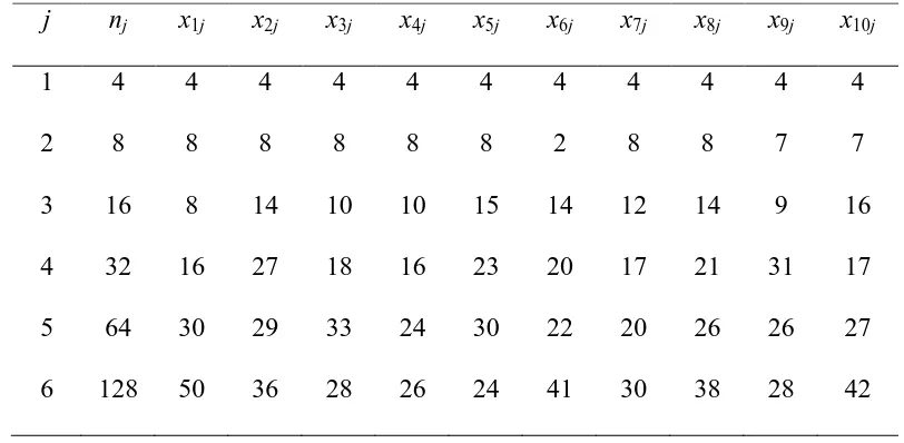
An observed dataset is presented in Table 1 for illustration; the second column 205
nj
( )
consists of the initial prey densities for j1,....,6 and the rest,(
x1,....,xj)
refer 206to the number of prey eaten by the predatorafter 24 hours. 207
The probability of observing xj prey items eaten out of njprey after 24 hours is 208
given by: 209
j x
n xh j
j
j
p p x n T a n x x
P
0, , 1 (5)
10
where pP
t a,Th
is given in Equation 2 for t 24 and therefore is implicitly 211dependent upon a and Th via (1). Assuming independence between the k replicates 212
in each experiment as well as between the different experiments, the likelihood of the 213
observed data X given the parameters
a,Th
after T 24 hours is written as 214follows: 215
j
h j j
h X a P x n a T
T a
L , , , , . (6)
216
Posterior Distribution
217
Equations 3, 4 and 6 give rise to the posterior distribution whose density is given as 218
follows: 219
k j
h h
j j
h X P x n a T a T
T
a, , , 12exp 1 2
(7)
220
The posterior density of interest (Equation 7) is not of a closed form due to its 221
normalising constant not being available explicitly. Therefore, in this study we 222
employed to a random walk Metropolis algorithm (Gamerman and Lopes 2006) to 223
draw samples from
a,Th X
.224
Bayesian Model Choice
225
Statistical inference, in general, is not limited to parameter estimation. Another 226
common goal is hypothesis testing, in which we are interested in discriminating 227
models in order to gain a better understanding of the structure of the statistical 228
model(s) of interest and facilitate for model-robust decision making. Here we are 229
interested in observing the extent to which the observed data support the scientific 230
hypothesis that the differential form of the disc equation is to be used when prey is 231
depleted during the functional response experiments. 232
Bayes Factors
11
The Bayesian approach to model selection (or discrimination) is based upon an 234
extension to the posterior distribution to include not only uncertainty regarding the 235
model parameters but also for the model itself. Consider the following framework: 236
suppose we observe data X and have a series of plausible models indexed by 237
W
w1,...., . Denote by w the vector of parameters associated with model Mw and 238
by w
X w
the likelihood of the observed data under model w. Then by specifying 239a prior distribution pk
w for the model parameters under each model and a prior 240probability for each model,p
Mw , we can derive the joint posterior distribution over 241both the model and parameter spaces, given by 242
w Mw X
w
X w
w w Mw , (8)
243
Assuming prior independence between Mw and w, the joint posterior distribution 244
can then be written down (using Bayes Theorem) as product of two components: 245
w w X
w w X
w X
, , (9)
246
where
w,Mw X
is the posterior distribution of the parameters under model Mw247
and
Mw X
denotes what we refer to as the “posterior model probability” which248
represents our beliefs, after observing data X , of what is the chance that model Mw
249
is the true model given that one of models 1,....,W is true. 250
Once these posterior model probabilities are obtained they can then be used to 251
discriminate between the competing models by computing the Bayes Factor which is 252
simply defined as the ratio of the posterior odds, i.e. the ratio of the posterior to the 253
prior model probability: 254
2
2
1 1
12
w w
w w
M M
X
M M
X BF
(10) 255
12
posterior odds = Bayes factor prior odds. 257
The value of the Bayes factor represents the relative likelihood of M1 to M2 and is of 258
practical appeal because its value is independent of the choice of the prior model 259
probabilities (see Kass and Raftery 1995). It is easy to see that when the models are 260
equally probable a priori so that
Mw 1
Mw 2
0.5the Bayes factor is 261equal to the posterior odds in favour of M1. The quantity
X Mw
for k 1,2 in 262(10) is obtained by integrating over the parameter space, 263
w
w w w w w
w X M d
M X
,
264
where w is the parameter vector under model Mw and w
w is its prior density. 265The term
X Mw
is the marginal probability of the data and is often called the 266marginal or integrated likelihood in the statistical literature while it is typically 267
referred to as the evidence in the physics and machine learning communities. The 268
Bayes factor is, therefore, a summary of the evidence provided by the data in favour 269
of one hypothesis represented by a statistical model as opposed to another. Note that 270
this formulation is completely general and does not require nested models, as is 271
typically the case with likelihood ratio tests. Additionally, no asymptotic justification 272
is required so that these results can be used for moderate sample sizes as well. 273
The marginal likelihoods are rarely available in analytic form. Therefore, in 274
practice if the number of parameters in each model is not very large (typically 2-5 275
parameters), then the marginal likelihoods and consequently the Bayes factors are 276
obtained via straightforward numerical integration. However, if the dimension of the 277
parameter vector θw is very large then computational tools such as trans dimensional
278
MCMC algorithms (Green 1995) can be used instead to explore the more complex 279
13 281
Results and Discussion
282
The functional response is a fundamental characteristic of predator-prey 283
systems. We have developed a hierarchical model which accounts for 284
heteroscedasticity and illustrated how to infer the parameters of interest (e.g. the 285
attack rate and the handling time) within a Bayesian framework using Markov Chain 286
Monte Carlo methods. In addition, we showed how one can assess competing 287
scientific hypotheses by investigating which model is mostly supported by the 288
experimental data. Generally, ODEs are frequently used in representing consumer-289
resource interactions and the outcome of such models is therefore of great interest to 290
researchers. Thus, we have made our computer code implementing the present 291
analysis in R (R Core team 2013) publicly available on http://www.maths.nott.ac.uk/ 292
~tk/files/functional_response/, to encourage and allow researchers to fit (and compare)
293
the proposed models to their datasets. 294
In practice, we often summarize the posterior distribution of the parameters by 295
calculating a variety of interpretable summary statistics such as posterior means, 296
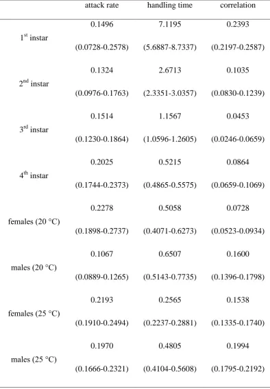
medians and credible intervals. The posterior means of both parameters of the disc 297
equation obtained are presented in Table 2. By inspecting the 95% credible intervals 298
we observe that the estimated attack rates were similar for all four larval stages of the 299
predator, indicating that the larvae have similar abilities to respond to increasing prey 300
densities. On the other hand, handling times decreased for the older larvae. This 301
further indicates an increase in the upper level of the response, leading older larvae to 302
a higher consumption of prey. Being larger gives them an advantage in handling prey. 303
At 20 °C, the attack rate for females was higher than those for males. This means that 304
14
satiated) the females have the ability to consume more prey items than the males. 306
However, comparison of handling times yielded no differences, indicating that both 307
sexes have similar maximum predation ability. Overall, at 20 °C we expect that 308
females, males and fourth instar larvae of P. quatuordecimpunctata to display the 309
higher predation ability among predators stages. This could be of great interest for 310
biological control practitioners, since these stages are to be preferred in potential 311
release of this predator in agroecosystems, allowing an influential decrease of aphid 312
pests. 313
Our results also showed that at the temperature of 25 °C there was a notable 314
difference of estimated handling times between males and females. This further 315
indicates that females might prey and subdue prey more efficiently and faster than 316
males. Moreover, handling time increased considerably as temperature decreased 317
from 25 °C to 20 °C for females, but not for males. According to Papanikolaou et al. 318
(2013), the fecundity of P. quatuordecimpunctata females is higher at 25 °C than 20 319
°C, where females of roughly 20-30 day-old exhibit their maximum reproductive 320
potential at 25 °C. As a consequence, higher energy requirements for egg production 321
lead them to higher consumption of prey. Additionally, attack rate for males was 322
lower at 20 °C than 25 °C unlike females, as it was not different among these 323
temperatures. Attack rate might follow a hump-shaped relationship with temperature 324
as it happens for the ladybird Coleomegilla maculata lengi DeGeer (Sentis et al. 325
2012). The two temperatures examined here might have been at the plateau of the 326
hump-shaped relationship with temperature for females and therefore no differences 327
occurred, whereas, for males was still increasing with temperature. 328
Although investigating the Pearson’s correlation between the estimated 329
15
literature, it is important to do so since this may reveal potential parameter non-331
identifiability issues as well as biological insights. Table 2 reveals a moderate but 332
statistically significant positive correlation between the estimated handling times and 333
the estimated attack rates of the predator, based on 95% credible intervals. This is 334
biologically intuitive since coccinellids are being highly voracious, especially larvae 335
which consume more prey items than they need for their development (Hodek et al. 336
2012). This trend may lead to a gradual increase of the handling time, as the attack 337
rate increases. 338
In a previous study (Papanikolaou et. al. 2011) the authors fitted the non-differential 339
form of the disc equation using a non-linear least squares approach, in order to 340
provide inference for the functional response of P. quatuordecimpunctata larvae. The 341
values of attack rates are notably lower than those estimated in the present analysis, 342
indicating that linearisation may induce estimation bias. The attack rate coefficient 343
illustrates the per capita prey consumption at low prey densities, indicating the initial 344
slope of the functional response curve. A biased estimate of this parameter leads to 345
underestimation of prey consumption at the lower prey densities, in which the 346
handling time is not the limiting factor of the predation. In addition, a high value of 347
the attack rate coefficient shows that the predator may exhibit stronger density-348
dependent predation behavior. In contrary, the values of the larvae handling times are 349
close to those estimated in the present analysis. Handling time depicts a more 350
complex behavior which includes a number of distinguish predator activities, such as 351
pursuing, subduing, eating and digesting a prey item. 352
353
354
Model Selection
16
We applied the proposed method in two cases: 356
a) Our hypothesis is translated into two different models, describing type II functional 357
responses; in particular 358
M1:
0 0
1 aT N aN dt t dN h 359
M2:
N aT aN dt t dN h 1 360
Note that the model M1 uses the functional response used Papanikolaou et al. (2011) 361
while M2 uses the hierarchical model that is proposed in Material and Methods. 362
b) In this case, our aim was to distinguish between type II and type III functional 363
responses, which is of importance in functional response studies (Juliano 2001), i.e.: 364
M2:
N aT aN dt t dN h 1 365
M3:
2 2
1 aT N aN dt t dN h , 366
where the model M3 describes type III functional responses. 367
In each cases, we assumed that both models are equally likely a priori and 368
consider Exponential prior distributions for both parameters, a Exp
, Th Exp
369. It is well known that the Bayes factor can be sensitive to the choice of model 370
parameter's prior distributions. Therefore, we computed the Bayes factor for a range 371
of different values of , namely, 0.01, 0.1, 1, and 10. We first computed the log of 372
the marginal likelihoods for both models via numerical integration and then the Bayes 373
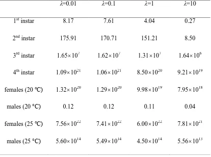
Factors of model M2 versus M1 in the first case and M2 versus M3 in the second case. 374
Table 3 and 4 shows the Bayes Factors of model M2 versus model M1 and M2versus 375
M3, respectively, for the different datasets and for different prior distributions. It is 376
17
M1 is to be preferred). Furthermore, the conclusions appear to be robust to the 378
different choice of . 379
Type II functional responses are frequent in nature, especially among 380
aphidophagous ladybirds (Hodek et al. 2012) and are typically descibed by Holling's 381
disc equation, one of the most commonly used models in ecology. Our study allowed 382
us to predict the efficiency of P. quatuordecimpunctata on a common and important 383
aphid species. Since biological control practitioners often rely on functional response 384
studies to design and use efficiently biocontrol agents, an accurate and non-biased 385
estimation of the functional response parameters is of crucial importance. The 386
approach developed here is towards that direction, for a more precise estimation of the 387
parameters that determine the shape of the functional response of a predator. Also, 388
functional response parameters of P. quatuordecimpunctata preying on A. fabae may 389
be incorporated in predator-prey models evaluating the population dynamics of the 390
study organisms. 391
From a statistical viewpoint routine Bayesian inference and model selection for 392
ODE-based models remains a challenge for a number of reasons which relate to the 393
need for solving the ODEs numerically. With respect to the former one may extend 394
our methods by utilising gradient-based information for the construction of efficient 395
MCMC proposals. The issue of model selection can be further explored by 396
methodology based upon thermodynamic integration (Friel and Pettitt 2008). Such an 397
approach is appealing in cases where numerical integration might be infeasible due to 398
the large number of parameters in the model, resulting in the evaluation of high-399
dimensional integrals. These are important directions for future research. 400
401
References
18
Beddington J. 1975. Mutual interference between parasites or predators and its effect 403
on searching efficiency. J. Anim. Ecol. 44(1):331-340. 404
Blackman, R.L. and V.F. Eastop. 2000. Aphids on the world's crops. An identification
405
and information guide. John Wiley & Sons. 406
Bolker, B. 2008. Ecological Models and Data in R,Princeton University Press. 407
Brooks, S., A. Gelman, G. Jones and X.L. Meng. 2011. Handbook of Markov Chain
408
Monte Carlo. Taylor & Francis US. 409
Englund, G., G. Ohlund, C.L. Hein and S. Diehl. 2011. Temperature dependence of 410
the functional response. Ecol. Lett. 14(9):914-921. 411
Fan, Y. and F.L. Petitt. 1994. Parameter estimation of the functional response. 412
Environ. Entomol. 23(4):785-794. 413
Fenlon & Faddy (2006) Modelling predation in functional response Ecol. Model. 198: 414
154-162. 415
Friel, N. and A.N. Pettitt. 2008. Marginal likelihood estimation via power posteriors. 416
J. R. Stat. Soc. B 70(3):589-607. 417
Gamerman, D. and H.F. Lopes. 2006. Markov Chain Monte Carlo: Stochastic
418
Simulation for Bayesian Inference. Chapman and Hall/CRC. 419
Gelman, A., G. Roberts and W. Gilks. 1996. Efficient metropolis jumping rules. In 420
Bernado, J.M. et al. (eds), BayesianStatistics, volume 5, page 599. OUP. 421
Gelman, A., W.R. Gilks and G. Roberts. 1997. Weak convergence and optimal 422
scaling of random walk Metropolis algorithms. Ann. Appl. Probab. 7(1):110-120. 423
Green, P.J. 1995. Reversible jump Markov chain Monte Carlo computation and 424
Bayesian model determination. Biometrika 82(4):711-732. 425
Hassell, M., J. Lawton and J. Beddington. 1977. Sigmoid functional responses by 426
19
Hastings, W. 1970. Monte Carlo samping methods using Markov chains and their 428
applications. Biometrika 57: 97-109. 429
Hodek, I., H.F. van Emden and A. Honěk. 2012. Ecology and Behaviour of the
430
Ladybird Beetles (Coccinellidae). Wiley-Blackwell. 431
Holling, C.S. 1959a. The components of predation as revealed by a study of small-432
mammal predation of the European pine sawfly. Can. Entomol. 91:293-320. 433
Holling, C.S. 1959b. Some characteristics of simple types of predation and parasitism. 434
Can. Entomol. 91:385-398. 435
Jeschke, J.M., M. Kopp and R. Tollrian. 2002. Predator functional responses: 436
discriminating between handling and digesting prey. Ecol. Monogr. 72(1):95-437
112. 438
Juliano, S.A. 2001. Nonlinear curve fitting: predation and functional response curves. 439
In: S.M. Scheiner and J. Gurevitch (eds), Design and analysis of ecological
440
experiments. Oxford University Press, Oxford, UK, p.p. 178-196. 441
Kass, R.E. and A.E. Raftery. 1995. Bayes factors. J. Am. Stat. Ass. 90: 773-795. 442
Livdahl, T.P. 1979. Evolution of handling time: the functional response of a predator 443
to the 450 density of sympatric and allopatric strains of prey. Evolution
444
33(2):765-768. 445
Livdahl, T.P. and A.E. Stiven. 1983. Statistical difficulties in the analysis of predator 446
functional response data. Can. Entomol. 115:1365-1370. 447
Metropolis, N., A.W. Rosenbluth, M.N. Rosenbluth, A.H. Teller and E. Teller. 1953. 448
Equation of State Calculations by Fast Computing Machines. J. Chem. Phys.
449
21:1087-1092. 450
Okuyama, T. 2012a. Flexible components of functional responses. J. Anim. Ecol.
451
20
Okuyama, T. 2012b. A likelihood approach for functional response models. Biol.
453
Contr. 60(2):103-107. 454
Papanikolaou, N.E., P.G. Milonas, D.C. Kontodimas, N. Demiris and Y.G. Matsinos. 455
2013. Temperature-dependent development, survival, longevity and fecundity of 456
Propyleaquatuordecimpunctata (Coleoptera: Coccinellidae). Ann. Entomol. Soc.
457
Am. 106(2):228-234. 458
Papanikolaou, N.E., A.F. Martinou, D.C. Kontodimas, Y.G. Matsinos and P.G. 459
Milonas. 2011. Functional responses of immature stages of Propylea
460
quatuordecimpunctata (Coleoptera: Coccinellidae) to Aphis fabae (Hemiptera: 461
Aphididae). Eur. J. Entomol. 108(3):391-395. 462
R Core Team. 2013. R: A Language and Environment for Statistical Computing.
463
Ripley, B.D. 1987. Stochastic simulation. John Wiley & Sons, Inc., New York, NY, 464
USA. 465
Rogers, D.J. 1972. Random search and insect population models. J. Anim. Ecol. 41: 466
369-383. 467
Sentis, A., J.L. Hemptinne and J. Brodeur. 2012. Using functional response modeling 468
to investigate the effect of temperature on predator feeding rate and energetic 469
efficiency. Oecologia 169(4):1117-1125. 470
Solomon, M. 1949. The natural control of animal populations. J. Anim. Ecol. 18(1):1-471
35. 472
Trexler, J., C. McCulloch and J. Travis. 1988. How can the functional response best 473
21
Table 1. Number of prey items consumed by Propylea quatuordecimpunctata
male adults for each trial (i=1,…,10). The experiment was conducted at 20 °C
for six different Aphis fabae prey densities (nij, j = 1, …, 6). Therefore, xij
denotes the count of consumed prey at the j-th density at the i-th trial.
j nj x1j x2j x3j x4j x5j x6j x7j x8j x9j x10j
1 4 4 4 4 4 4 4 4 4 4 4
2 8 8 8 8 8 8 2 8 8 7 7
3 16 8 14 10 10 15 14 12 14 9 16
4 32 16 27 18 16 23 20 17 21 31 17
5 64 30 29 33 24 30 22 20 26 26 27
6 128 50 36 28 26 24 41 30 38 28 42
[image:21.595.93.499.181.380.2]22
Table 2. Parameter values of Holling’s disc equation obtained as posterior
means (95% Credible Intervals), and the correlation of attack rate and handling
time (95% Credible Intervals).
attack rate handling time correlation
1st instar
0.1496
(0.0728-0.2578)
7.1195
(5.6887-8.7337)
0.2393
(0.2197-0.2587)
2nd instar
0.1324
(0.0976-0.1763)
2.6713
(2.3351-3.0357)
0.1035
(0.0830-0.1239)
3rd instar
0.1514
(0.1230-0.1864)
1.1567
(1.0596-1.2605)
0.0453
(0.0246-0.0659)
4th instar
0.2025
(0.1744-0.2373)
0.5215
(0.4865-0.5575)
0.0864
(0.0659-0.1069)
females (20 °C)
0.2278
(0.1898-0.2737)
0.5058
(0.4071-0.6273)
0.0728
(0.0523-0.0934)
males (20 °C)
0.1067
(0.0889-0.1265)
0.6507
(0.5143-0.7735)
0.1600
(0.1396-0.1798)
females (25 °C)
0.2193
(0.1910-0.2494)
0.2565
(0.2237-0.2881)
0.1538
(0.1335-0.1740)
males (25 °C)
0.1970
(0.1666-0.2321)
0.4805
(0.4104-0.5608)
0.1994
(0.1795-0.2192)
[image:22.595.113.508.155.724.2]23
Table 3. The Bayes Factor of M2 versus M1 for different values of the prior's
hyperparameter λ.
λ=0.01 λ=0.1 λ=1 λ=10
1st instar 8.17 7.61 4.04 0.27
2nd instar 175.91 170.71 151.21 8.50
3rd instar 1.65107 1.62107 1.31107 1.64106
4th instar 1.091021 1.061021 8.501020 9.211019
females (20 °C) 1.321020 1.291020 9.981019 7.951018
males (20 °C) 0.12 0.12 0.11 0.04
females (25 °C) 7.561022 7.411022 6.001022 7.811021
males (25 °C) 5.601014 5.491014 4.501014 5.561013
477
[image:23.595.98.512.127.435.2]24
Table 4. The Bayes Factor of M2 versus M3 for different values of the prior's
hyperparameter λ.
λ=0.01 λ=0.1 λ=1 λ=10
1st instar 1.47 1.53 2.08 1.55
2nd instar 29.83 29.93 30.67 20.91
3rd instar 56.41 55.56 47.78 10.70
4th instar 1.69 1.67 1.43 0.30
females (20 °C) 132614 130522 111268 22586
males (20 °C) 2.641014 2.611014 2.331014 7.381013
females (25 °C) 614829 604344 508693 91812
males (25 °C) 6309 6230 5497 1559
[image:24.595.97.512.127.434.2]