EFFECTIVE TERMINATION TECHNIQUES
Nick I. Cropper
A Thesis Submitted for the Degree of PhD
at the
University of St Andrews
1997
Full metadata for this item is available in
St Andrews Research Repository
at:
http://research-repository.st-andrews.ac.uk/
Please use this identifier to cite or link to this item:
http://hdl.handle.net/10023/13453
Effective Termination Techniques
Nick I Cropper
30 September 1996
Submitted in partial fulfillment of the requirements for the degree of Doctor of Philosophy in Computer Science
ProQuest Number: 10167225
All rights reserved
INFORMATION TO ALL USERS
The quality of this reproduction is dependent upon the quality of the copy submitted.
In the unlikely event that the author did not send a com plete manuscript and there are missing pages, these will be noted. Also, if material had to be removed,
a note will indicate the deletion.
uest
ProQuest 10167225
Published by ProQuest LLC (2017). Copyright of the Dissertation is held by the Author.
All rights reserved.
This work is protected against unauthorized copying under Title 17, United States C ode Microform Edition © ProQuest LLC.
ProQuest LLC.
789 East Eisenhower Parkway P.Q. Box 1346
\ V
I, Nick Cropper, hereby certify that this thesis, which is approximately 30 000 words in length, has been written by me, that it is the record of work carried out by me, and that it has not been submitted in any previous application for a higher degree.
date 1^ / 3 / 4 1_____ signature of candidate __-
---I was admitted as a research student in October 1992 and as a candidate for the degree of doctor of philosophy in October 1993; the higher study for which this is a record was carried out in the University of St Andrews between 1992 and 1995.
date signature of candidate . --- :—
I hereby certify that the candidate has fulfilled the conditions of the Res olution and Regulations appropriate for the degree of doctor of philosophy in the University of St Andrews and that the candidate is qualified to submit this thesis in application for that degree.
date / 2. signature of supervisor____
In submitting this thesis to the University of St Andrews I understand that I am giving permission for it to be made available for use in accordance with the regulations of the University Library for the time being in force, subject to any copyright vested in the work not being affected thereby. I also understand that the title and abstract will be published, and that a copy of the work may be made and supplied to any bona fide library or research worker.
Order leads to all the virtues!
but what leads to order?
Georg Christoph Lichtenherg
Abstract
An important property of term rewriting systems is termination: the guar antee that every rewrite sequence is finite. This thesis is concerned with orderings used for proving termination, in particular the Knuth-Bendix and polynomial orderings.
First, two methods for generating termination orderings are enhanced. The Knuth-Bendix ordering algorithm incrementally generates numeric and symbolic constraints that are sufficient for the termination of the rewrite system being constructed. The KB ordering algorithm requires an efficient linear constraint solver that detects the nature of degeneracy in the solution space, and for this a revised method of complete description is presented that eliminates the space redundancy that crippled previous implementations.
Polynomial orderings are more powerful than Knuth-Bendix orderings, but are usually much harder to generate. Rewrite systems consisting of only a handful of rules can overwhelm existing search techniques due to the combinatorial complexity. A genetic algorithm is applied with some success.
Second, a subset of the family of polynomial orderings is analysed. The polynomial orderings on terms in two unary function symbols are fully re solved into simpler orderings. Thus it is shown that most of the complexity of polynomial orderings is redundant. The order type (logical invariant), either r or A (numeric invariant), and precedence is calculated for each polynomial ordering. The invariants correspond in a natural way to the parameters of the orderings, and so the tabulated results can be used to convert easily between polynomial orderings and more tangible orderings.
The orderings of order type are two of the recursive path orderings. All of the other polynomial orderings are of order type w or ufi and each can be expressed as a lexicographic combination of r (weight), A (matrix), and lexicographic (dictionary) orderings.
Acknowledgement s
I would like to thank my supervisor, Ursula Martin, for guiding me through the intractabilities of termination and for the many stimulating and insightful discussions. I am very grateful to the termination community, particularly the participants of the termination workshops, with particular thanks to Joachim Steinbach, Jürgen Giesl, and Elizabeth Scott.
It was a pleasure to study in the Computer Science Division, and I would like to thank my colleagues in St Andrews and York who supported this work.
I must also take this opportunity to thank my friends and family who have been so tolerant during this indulgent but immensely rewarding period of my life.
Contents
0 Introd uction 1
0.0 Terminating P ro cesses... 1
0.1 Termination in P r a c tic e ... 3
0.2 Term R ew riting... 5
0.3 Proving T erm ination... 10
0.3.0 Monadic T e rm s... 14
0.3.1 Order In v a ria n ts... 15
0.3.2 Polynomial A n a ly sis... 16
0.4 Document S tru c tu re ... 18
1 Prelim inaries 20 1.0 N otation... 20
1.1 T e r m s ... 20
1.2 Term R ew riting... 21
1.3 O rd erin g s... 23
1.3.0 Weight O rderings... 26
1.3.1 Knuth-Bendix O rderings... 26
1.3.2 Recursive Path O rd erin g s... 27
1.3.3 Polynomial O rd e rin g s... 27
2 K nuth-B endix O rdering A lgorithm 31 2.0 Introduction... 31
2.1 P relim inaries... 32
2.1.0 Vectors and M atrices... 32
Contents viii
2.1.1 Linear In equalities... 34
2.1.2 Hyperplanes... 36
2.1.3 Cones and Polyhedra... 36
2.1.4 Double D escription... 37
2.1.5 Degeneracy ... 37
2.2 Incremental KB Ordering A lg o rith m ... 38
2.3 Method of Complete D escrip tio n ... 41
2.4 Illustration of Redundancy in M C D ... 42
2.5 Removing Redundancy from the M C D ... 47
2.6 Revised M C D ... 49
2.7 C onclusions... 49
3 G enetic T erm ination 52 3.0 Introduction... 52
3.1 Termination by Polynomial O rdering... 55
3.1.0 Method of BenCherifa & L escan n e... 56
3.1.1 Method of S teinbach... 57
3.1.2 Method of G iesl... 58
3.1.3 Gradients M e th o d ... 58
3.2 Genetic A lgorithm s... 60
3.2.0 E n c o d in g ... 60
3.2.1 Fitness... 62
3.2.2 Selection... 62
3.2.3 R ecom bination... 63
3.2.4 M u ta tio n ... 64
3.2.5 Trials ... 64
3.3 Further D evelopm ents... 67
Contents ix
3.3.1 Numerical O ptim isation... 70
3.4 Conclusions... 71
4 A nalysis o f P olynom ial O rderings 73 4.0 Introduction... 73
4.1 Polynomial Orderings on Monadic Term s... 73
4.2 Ordering Invariants... 76
4.2.0 Order Types ... 77
4.2.1 Numeric Invariants... 78
4.2.2 Lexicographic E x te n sio n s... 80
4.3 Two Unary Function Sym bols... 82
4.3.0 Order Types ... 85
4.3.1 Numeric Invariants... 89
4.3.2 Lexicographic E x te n sio n s... 92
4.3.3 Summary for Two Unary Function S y m b o ls... 97
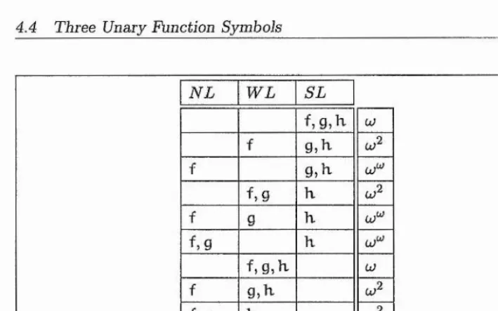
4.4 Three Unary Function S ym bols... 99
4.4.0 Order Type lu... 100
4.4.1 Order Type ...101
4.4.2 Order Type ...103
4.5 Further D evelopm ents...104
5 C onclusions 106 5.0 S u m m a ry ...106
5.1 Pipeline of Ordering F a m ilie s...107
5.2 Extending the O rderings... 107
5.3 Test B e d ... 108
List of Tables
0.0 Order types of total simplification orderings on binary strings. 16 0.1 Polynomial orderings on binary monadic terms (summary). . 17
List of Figures
0.0 A nested loop (in Pascal) ... 3
2.0 Incremental Knuth-Bendix Ordering A lgorithm ... 41
2.1 Method of Complete D escrip tio n ... 42
2.2 Revised Method of Complete Description ... 49
3.0 Partitioning the hypercube... 55
3.1 Well-foundedness of polynomial orderings... 57
3.2 Genetic Algorithm for T erm ination... 60
Notation
Abbreviations Page refs for symbols
a.k.a. also known as == 5
cf. compare —1> 22
e.g. for example 22
etc. and so on ^ pol 74
i.e. that is 78
iff if and only if 79
resp. respectively >Rilrx 81
s.t. such that 4 83
wlog without loss of generality
w.r.t. with respect to
0 Introduction
In this chapter we describe what is meant by ‘termination’, set a context for the subsequent discussion, and give an overview of the document.
0.0 Term inating Processes
Let us begin by considering the progress of a hypothetical slide show. Sup pose the projectionist has a number of boxes of slides, each box contain ing slides numbered sequentially from 0. For this viewing the projection ist will present one box of slides, projecting the slides in reverse ordet: 50, (gQ — 1), ...,1,0. Before the first slide is projected, all the audience knows regarding running length is that the first slide will be indexed by a positive whole number, that each successive index will be smaller, and that no slide has a negative index. Thus the audience deduces that only a finite number of slides will be shown and therefore the viewing must eventually terminate.
If the projectionist promises that no slide will be projected for longer than some upper bound, five minutes say, then as soon as the index of the first slide (sq) is known, an upper bound ((sq + 1) x 5 minutes) for the entire
viewing is known. This upper bound holds even if the projectionist omits some slides from the box.
Now suppose that the projectionist intends to present 2 boxes of slides:
51, (si — 1),..., 1,0, So, (sq — 1),..., 1,0. The audience can no longer place
0.0 Terminating Processes
that ‘time until termination’ can be bounded. Nevertheless, the audience can still characterise the terminating nature of the viewing; the ‘double box’ viewing is simply the sequential composition of two versions of the ‘single box’ viewing. Logicians say the ‘single box’ sequence (natural numbers under the usual ordering) has ‘order-type’ w. (This terminology will be formally defined in Chapter 1.) The order-type of the ‘double box’ sequence (• • • >
2 > l > 0 > - ' - >2 > l > 0) i s w4-w, written w.2.
Finally suppose that the projectionist will present an unspecified number of boxes of slides, but that each box is indexed in the same manner as the slides. Before arriving at the viewing, the audience are ignorant not only of the number of slides in each box, but also of the number of boxes. The sequence of boxes will have order-type w, and the slides of each box will have order type uj, so the termination nature of the viewing can be characterised by w.w, written (Although these order-types are daunting for the pro jectionist’s audience and yet ‘tiny’ in comparison to those sometimes used in termination practice, they are roughly as large as we will find useful in the sequel.)
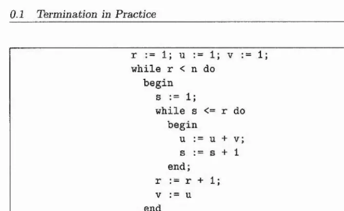
In 1949 Alan Turing used order-types to prove the termination of a sec tion of computer program, represented in a modern programming language in Figure 0.0. Turing used
“a;^.(n — r) -{- o).(i— s) -f fc”
as a sequentially decreasing expression to demonstrate its termination.® Noticing that the expression pair (n — r, r — s) follows the same sequence as the pair {box-index, slide-index) from the example above, we can conclude that the termination of the program is also characterised by the order-type
“Turing suggested 2“’° could be substituted for w since that was an upper bound for the
variables the particular computer could represent. The variable k was due to an expression
0.1 Termination in Practice
r := 1; u := 1 V := 1; while r < n do
begin s := 1;
while s <= r do begin
u := u + v ;
s := s + 1 end;
r := r + 1;
V : = u
end
Figure 0.0: A nested loop (in Pascal)
ufi. In abstracting away the slides and Pascal code, we can focus on the expressions that characterise the advancement towards termination. If we can prove that such an expression follows (or is contained in) a decreasing sequence that cannot decrease indefinitely, we have proved termination.
0.1 Term ination in Practice
[image:18.612.84.437.80.296.2]0.1 Termination in Practice
In practice, however, much computation is achieved without the de
velopers being aware of a theory of termination as such. Single-threaded programs are often assured terminating using little more than the well- foundedness of the natural numbers. Multi-threaded programs can employ techniques such as time-outs to ‘pull the plug’ on tardy processes.
For safety-critical software a degree of termination assurance can be im posed by the project manager. Part of the design rationale for the SPARK ADA language ([CJM+92]) is to make termination arguments clearer by banning certain ‘dangerous’ constructs such as got os that are in the full ADA language. Currie’s NewSpeak ([Cur89]) goes all the way by excluding unbounded loops entirely, at the cost of Turing completeness.
One application area targeted by such languages is hard real-time sys tems, where satisfying temporal constraints is as important as functional cor rectness. For such software it is extremely desirable to have at compile time bounds on both its space and time requirements. This necessitates bounds on depth of calls to sub-programs as well as bounds on all program loops. Whereas NewSpeak achieves this via a restricted syntax, SPARK ADA is a strictly more expressive language and instead aims to facilitate proof that requirements are met. Hence such systems require the proof of termination to be strengthened by proof that the components terminate within given time bounds.
0.2 Term Rewriting
evaluation, so a functional program may be evaluated as a non-deterministic term rewriting system.
These are approaches designed to ease the task of avoiding non-termination in certain computer systems, but as the systems become larger and more complex, and the potential costs of system failure rise, it becomes increas ingly important to prove the correctness of the system. In turn we need more powerful and sophisticated theorem provers, which need to be partially auto mated, and whose processes therefore need to be proved terminating. Here we are concerned with the term rewriting ‘equational reasoning engine’ for automated theorem proving.
0.2 Term R ew riting
Equations play an important part in the mathematical sciences. They are used, for example, to specify algebraic properties of data structures. We may want to specify that all the stacks in a computer system have the property pop(push(e, s)) = s, for instance.^ The set of such defining equations for a data type form the axioms of the data type’s equational theory. Part of the process of verification, where the specification is examined to establish if it captures those properties that were intended (and does not entail proper ties that are undesired), involves checking that equations identified as being important to the system being specified can be derived from the defining equations. For example, after defining the l i s t data type we may wish to verify that they have the property reverse(reverse(/)) = I. Formal reasoning about specifications is just one example where we wish to employ automation to check that propositions are theorems of an equational theory.
In [Bir35] Birkhoff showed that the rules
0.2 Term Rewriting
(refiexivity) -— (symmetry) j- r — (transitivity)
^ (context) . ^ (substitution)
f { . . . t . . . ) = f { . . . u . . . ) t(7 = u a
are complete for first order (universally quantified) equational reasoning; the equations derivable from a given set of equational axioms are exactly those equations that hold in all models of the axioms. (We focus our attention on first-order universally quantified clauses; much of what will be discussed applies to the various extensions that exist.)
Using these derivation rules, a proposition Ihs = rhs is a theorem of a given equational theory if the left-hand side can be rewritten to the right- hand side by applying the derivation rules to the axioms, so that a derivation chain Ihs = Ihs' = • • • = rhs can be formed.
As it stands, the process just described cannot be automated effectively. First, the derivation rules of refiexivity and symmetry can prevent any pro gress being made, Ihs = Ihs' = Ihs = Ihs' = Ihs' = • • •. Second, there is no goal-direction for the next link in the derivation chain, so a less trivial chain may look like it is making progress, but it may never reach the right-hand side, Ihs = Ihs' = Ihs" = - ». That is, the search tree is too wide and too deep.
To tackle these problems, each axiom li = can be turned into a ‘direc ted equation’, li -> r^, known as a rewrite rule. The set of axioms {l{ —> r*} now defines the rewrite relation - 4 as the smallest transitive binary relation
containing ~t> and closed under context and substitution.
t u u V , . . . V
0.2 Term Rewriting
t u ,(context) , . --- (substitution)t u / 1 X
f { . . . t . . . ) - ^ f { . . . u . . . ) t a ua
If there exists a chain Ihs -> Ihs' —>••••—> rhs then Ihs = rhs is a theorem of the theory being examined. Therefore the set of rewrite rules -> provides a semi-decision procedure for the original equational theory; if rewriting relates two terms then those terms are equationally related, but the converse does not necessarily hold.
The rewriting process may be proved terminating by showing that the rewrite relation -> is well-founded, i.e. it admits no infinite chains. If the process is terminating it can be fully automated; apply rewrite rules to Ihs and rhs until no more rewrites can be applied, producing terms Ihs' and rhs'\ if Ihs' = rhs' then the theorem Ihs = rhs is proved.
A terminating rewrite system^ solves the problem of depth since all chains are finite. However, two problems remain. The search tree may still be too wide; a given term may rewrite to many different final forms (called normal forms) and at each rewrite the system has no way of determining which possible chain may be most fruitful. Second, by making the axioms mono-directional the rewrite procedure may have lost some of the power of the original equational system. In their seminal paper [KB67] Knuth and Bendix showed that these problems were one and the same, as represented schematically below.
We would like to prove that to = ^4 is a theorem, but the rewriting of to and
0.2 Term Rewriting
t4 stop at ti and ts respectively; the rewrite relation is ‘missing’ the ability
to relate ti and directly.
The Knuth-Bendix completion procedure ([KB67]) takes a terminating rule set and detects pairs of terms t, t' such that t ^ t' but which cannot be related directly. A new rule, either t —> t' or t' t, is added to the system if the termination property can be maintained. This is represented on the diagram as
where ^3 -> ti is the new rule to be added. The augmented system containing the new rule is then tested for more rules to be added. If this procedure of adding pairs terminates then the augmented system is confluent: any two chains from a given term re-join at a common descendent. Since the property of termination has been maintained, any such system is convergent; all terms have unique normal forms. Thus, if successful, completion provides a complete decision procedure since two terms are equal if and only if their normal forms are the same.^
As described in the following section, termination of term rewriting sys tems is usually proved by finding a terminating relation (termination or dering) that includes the rewrite relation. For the purpose of a completion procedure, there are several important aspects to the termination ordering used.
First, the ordering has to contain each term pair in the rule set. This is
0.2 Term Rewriting_______________________________________________9
unitary termination: all term pairs may be examined before any constraints are placed on a termination ordering. To be of practical use for a completion procedure, minimal time should be required to determine whether a par ticular class of orderings (e.g. Knuth-Bendix orderings) is able to correctly orient each of the rewrite rules. If a class of orderings is unsuccessfully ap plied, another class (e.g. polynomial orderings) may be tried. A completion procedure often generates many term pairs and so the ordering technique may be required to consider many sets of term pairs. Part of the reason that term rewriting is increasingly popular as an efficient proof mechanism is because current termination techniques are often able to fulfill these require ments. However, if we are to increase the range and speed of rewrite-based automated theorem provers we need to look at how termination techniques can be made more effective.
Second, as completion proceeds the rule set will in general grow, poten tially to an unlimited number of term pairs, with new rules being integrated one rule at a time. This is incremental termination: the termination order ing has already been constrained before the new term pairs are available for consideration. It is clearly desirable to employ an incremental termination technique; one that can minimally augment its constraint data to integrate the new constraints rather than throw away previous data to start from scratch.
0.3 Proving Termination 10
employed can re-use information from the first orientation instead of having to start afresh with the second orientation. More difficult in general is the ability to optimally decrement the constraints, so that if a rule is removed from the rule set the termination technique isn’t unnecessarily constrained. It is usually more practical either to proceed with the unnecessary constraints or to restart the process of proving the current system terminates.
Fourth, different orderings may orient candidate term pairs in oppos ing directions (or allow either orientation). Whichever orientation is taken when the term pair becomes a new rewrite rule may affect the success of the completion procedure. Orienting a rule in one direction may cause the completion procedure to generate infinitely many new rules when orienting in the other direction may have led to a finite convergent rewriting system (see for example [Les86]).
Finally, the orientation of rules can affect the efficiency of the resulting rewrite relation, meaning that the number of rewrite steps applied to a given term may be different in two semantically equivalent rewriting systems. It may be possible to attribute upper bounds to the derivations of the rewriting system knowing properties of the containing termination ordering (its order type).
0.3 Proving Term ination
Any (non-random) terminating process progresses ‘closer’ to termination. The task of proving termination is to find the appropriate ‘measure’. If a rewrite relation^ is terminating then there exists a well-founded rewrite relation that contains it: for example, the rewrite relation itself. Thus the
0.3 Proving Termination__________________________________________H
task of proving termination of a rewrite relation - 4 defined by —> is to find
a rewrite relation -4 ' known to be well-founded such that - 4 Ç -4 '. The relation -4' is called a termination ordering, and is usually written >*-. Prom the formulation of - 4 it suffices to show that Ç where — is the
(possibly infinite) set of rewrite rules derived from -t> by instantiating all variables with ground terms.
The problem of proving termination of a rewriting system can be re duced to the halting problem and so is undecidable, even for one-rule sys tems with only unary function symbols. Therefore the standard approach is try a certain family of orderings, and if unsuccessful to find a member suitable for proving termination, try a different family of orderings. In the literature there appear formulations for many families of termination or derings (for example, Knuth-Bendix orderings [KB67, Mar87], polynomial orderings [MN70, Lan75] [Ste94] [BL87b, CL92], recursive path orderings [KL80], transformation orderings [BL87a], subterm path orderings [Pla78], and recursive decomposition orderings [Les84]).
These families of orderings can be roughly grouped into two classes: syntactic orderings and semantic orderings. A syntactic ordering compares terms by the syntactic structure of the term tree, typically examining first the function symbol at the root and then recursively examining the sub-trees. The task of proving termination by such an ordering is to find an appropriate precedence: the ordering on function symbols. The recursive path orderings (formulated on p 27) are an important family of syntactic orderings. Stein bach examined a variety of such orderings in [Ste88] and found that many seemingly disparate families produced the same orderings when they were total (i.e. sufficiently defined to compare all terms).
0.3 Proving Termination 12
monotonie algebra® {A, >a) and then compares the resulting elements ac cording to >A- The task of proving termination by such an ordering is to find an appropriate interpretation of the function symbols so that the inter preted terms are decreasing in the underlying algebra:
t u
w >A
M
We will concentrate on two families of so-called ‘semantic’ orderings; Knuth-Bendix orderings and polynomial orderings. At the heart of a Knuth- Bendix ordering (formulated on p 26) is a weight ordering: function symbols are assigned non-negative weights, and terms are oriented by comparing weights. This is extended to non-ground terms by assigning a positive weight to all variables and requiring the multiset of variables in a term to be a sub multiset of all terms greater than that term. To compare terms with equal weights, the ordering is supplemented with a precedence (ordering on the function symbols) so that equal-weight terms are compared by their root symbols and then their subterms.
Knuth-Bendix orderings are popular due to their relative simplicity. When manually looking for an appropriate ordering it is often possible to make a good judgement by inspection alone as to whether to try the Knuth-Bendix family. Similarly for an automated tool, it is computationally easy to derive the constraints that a feasible KB ordering would need to satisfy. Indeed, Martin gave a complete decision procedure in [Mar87] to determine whether or not a given rewriting system is KB terminating. For these reasons, KB orderings are appropriate as the ‘first hammer’ when seeking to prove ter mination. Since their power is limited (due to their ‘flat’ interpretation of
0.3 Proving Termination__________________________________________3^
terms and the restriction on occurrences of variables) there need to be more sophisticated ordering families in the line of attack.
A polynomial ordering is defined by assigning polynomial functions over a domain, N say, to each function symbol. (See p 53 for an example.) For ground terms this is like a weight ordering, and non-ground terms are com pared by examining whether one dominates the other over a sub-domain that includes the values of all ground terms.
The search space for polynomial orderings is far larger than that for Knuth-Bendix orderings, and the relationship between the interpretation of function symbols and the resulting orientation of terms is much less intuitive. The hunt for a suitable polynomial ordering usually takes the form of
• restrict the form of polynomials to be considered, then
• search the polynomials of that form until a successful combination of interpretations is found.
0.3 Proving Termination__________________________________________W
0 . 3 . 0 M o n a d i c T e r m s
Monadic terms are constructed from unary function symbols, and so are iso
morphic to strings. For example, we can swap between thinking of f(f(g(æ))) and ffg.
Finding an interpretation such that the defined ordering contains all pairs of the rewrite relation is far from trivial for general terms (see [BL87b, Ste94]). However, we will see that, on monadic terms at least, polynomial orderings are much simpler than we might suppose. In fact we are able to classify them in terms of certain invariants explained below.
Although polynomial orderings on monadic terms are in only one vari able, there are unboundedly many parameters to set, and the author ex pected to see a great variety of orderings. In addition, it was unclear how the parameters of the interpretations related to the resulting ordering. Not only has much of the complexity of the interpretations proved redundant, but the properties of each ordering follow naturally and simply from the few significant parameters.
Knowing the properties of the available orderings is important when se lecting an ordering family in an attempt to prove a rewrite system is ter minating. Different families of orderings may have orderings in common, for example the recursive path orderings are common to several families. Indeed several independent formulations for recursive path orderings have been shown to be equivalent ([Les81]). Even with respect to a single for mulation, an ordering may have unboundedly many definitions. For ex ample, if a Knuth-Bendix ordering is defined by the weight assignment {wta = wi, wtb — W2} then, since the relative rather than absolute weights
are significant, the same ordering is defined by {wta = pwi, wtb = PW2}
0.3 Proving Termination__________________________________________15
On the other hand, by an appropriate choice of weights we can produce con
tinuum many distinct Knuth-Bendix orderings, as shown in [Mar93]. Clearly it is unsatisfactory to classify orderings solely by their formulation family, and we look to more fundamental characterisations of orderings: ordering invariants.
0 . 3 . 1 O r d e r I n v a r i a n t s
Two ordered sets are order-isomorphic if there is an order-preserving bijection between them. Just as cardinality is an abstraction over size, order type is an abstraction over order-isomorphism. Every well-founded total ordering (well-ordering) is order-isomorphic to an ordinal - its order type (logical invariant). More than simply a coarse tool for separating orderings, order types provide a logical measure of the reduction ‘power’ of total orderings. If a well-ordering >- with order type 0 contains a rewrite system 7Z (thus proving 7Z is terminating) then 0 can be related to the derivation complexity of 7Z (see [Cic90, Hof92]), which in turn can be related to the proof theoretic and algorithmic complexities of the relation being computed by 7Z (see [Wai93]).
In [MS93] detailed results are obtained for simple conditions determining the order types of total termination orderings on binary strings. Martin and Scott show that any total termination ordering on strings in two letters, say a and b with a b, has order type oj, cj^, or according to Table 0.0. In addition they show that the only such orderings of order type are the recursive path orderings.
0.3 Proving Termination 16
Table 0.0: Order types of total simplification orderings on binary strings.
Conditions Order Type
b-^ >- a for some j G N, w
a F- b'^ for all j E N and both b*a >- ab for some k E N and ab* b a for some k E N,
a F- for all j E N and
either ab X b*a for all /e G N or b a >- ab* for all k e N.
particular weight pre-order such that >- = • • •)• For order type the numeric invariant is a real number A > 0 that identifies the particular matrix pre-order such that >- = (^rl • • •) (where r = 0). These pre-orders are considerably easier to work with than polynomial orderings, and are detailed in Section 4.2. One of the surprising results of this work is that for almost all polynomial orderings on monadic terms in two function symbols we are able to describe the orderings completely: they are the extensions of these pre-orders with the standard lexicographic orderings from the right
0 . 3 . 2 P o l y n o m i a l A n a l y s i s
In Section 4.3.0 the main results of the polynomial analysis are presented in three parts: the order types, the numeric invariants, and the lexicographic combination equivalents. These may be summarised as follows.
Let y-poi be a polynomial ordering on monadic terms T({f,
g } , { v } )
defined by the interpretationsW (^) ■ GmZ™ H f diz -F «0, • • • Oo ^ 0, m > 1,
0.3 Proving Termination 17
Table 0.1: Polynomial orderings on binary monadic terms (summary).
Parameters LexicographicCombination OrderType InvariantNumeric
^polA m ^ n > 1 (fc r ; !>'“ ''> U) T = ^Inm
^ polB m > n = 1, b i > 1 (fc r ; k A l X = m
ypolC m > n — 1, b i = 1, 6o > 0 rpo LO'^
-^polD m — n = 1, a i ^ 6 i > 1 U) ^ _ In fei.Inai
^polE m = n = 1, b\ 1, 6o > 0 Up' A — a \
^polF m = n = 1, — 1, ao bo > 0 U) r = ^an
and [v|(a;) = x, such that f(v) ypoi g(v) ^poi v. The set of all such orderings is partitioned into subsets '^poiA'> '^polCi '^polD^ ^polE^ and ^poiFi uud the properties of the orderings are summarised in Table 0.1.
Thus we see that almost all the properties of the ordering are determined by the degree and coefficient of the leading monomial. Moreover, apart from two recursive path orderings, all the effectiveness of polynomial orderings can be obtained using linear interpretations only. These theoretical results tie in nicely with the experimental results of Steinbach in [Ste94] where he found a significant proportion of term rewriting systems orderable by general polynomial orderings could also be ordered by his so-called simple-mixed polynomial orderings.
We can illustrate some of the results of this work by examples:
0. |fl(a:) = Zx^^ 4- H- 1 and |[g]](z) = -f -f 9x
From row >-poiA we see that this is simply a weight ordering, with f having weight In 4 and g having weight In 3, extended with the lexico graphic ordering having g > f.
1. [f]](z;) = a; 4- 3 and [gl(a;) = æ 4- 2
0.4 Document Structure__________________________________________
having weights 3 and 2 respectively.
2. [fl(a;) = 4a; + 1 and [g]|(a;) = x -h 2
This is a so-called A ordering (defined in Section 4.2) as shown in row
>-polE- It has order type uP and in this case A = 4. In fact the leading coefficient of [f|(a;) is the only significant parameter.
3. |f](a;) = x"^ + 4 x-\-\ and |g|(ic) ~ x + 2
This is the standard (i.e. from the left) recursive path ordering (rpo) with f greater than g in the precedence. In fact we will see in Sec tion 4.3.0 that the same ordering is given whenever the interpretation of g has leading monomial x (i.e. |g | is strongly linear) and the leading index of the interpretation of f is greater than 1 (i.e. |f] is non-linear).
4. |fl(rc) = 3æ^ and |g](a;) = 5a; + 1
This is also a A ordering, from row )^pow^ even though the interpret ations are of completely different form to those in example 2. In fact it is exactly the same ordering with a lexicographic extension! If we use the ordering in example 2 extended with a lexicographic ordering having g D> f then the interpretations in this example are completely redundant.
0.4 D ocum ent Structure
0.4 Document Structure__________________________________________ W
1 Preliminaries
This chapter introduces most of the notation and concepts re quired for subsequent chapters. Puller accounts of term rewriting and termination can be found in [DJ90, Klo87, Pla93, JL87].
1.0 N otation
The set of natural numbers {0,1,2,3,...} is denoted N and the set of positive natural numbers {1,2,3,...} is denoted % . The set of real numbers (resp., positive real numbers) is denoted M (resp., R+). If A is a set then V{A) denotes the power set of A. The cardinality of a set A is denoted #(A ).
An ascending sequence denotes the empty sequence if j < i, so ( a i,... ,an) is the empty tuple if n < 1. For convenience a denotes a tuple (a i,... ,On) where n should be clear from the context. The set of n-length tuples over a set A is denoted A” , and the set of non-negative-length tuples is denoted A~^.
1.1 Terms
Let T he a finite set of function symbols and V be a countable set of vari ables. Each function symbol / is associated with a natural number, its arity ar(/) G N, signifying the number of arguments taken by the function. Func
tion symbols of arity 0, 1, 2, and 3 are described respectively as constant^ unary, binary, and ternary. In this document we will consider only finite sets of function symbols, each having fixed arity. Where convenient we will
1.2 Term Rewriting______________________________________________21
reserve the symbols f, g, K, /, g, h, /i, /2, • ■ • to denote function symbols and v ,x ,y ,z ,v i,V2, . .. to denote variables. (We assume an infinite supply of
variables so that we never run out of new names when we come to renaming variables, but it is even more convenient to think of the set V as being finite.)
The set of term s T(JF, V) is the set of variables V closed under construc tion by JF as f { t i , . . . ,tn), where n is the arity o î f E P. (If / is a constant then the empty brackets are elided.) The number of occurrences of a function symbol / in a term t is denoted # ( /,t) , and similarly for variables. The set of ground terms T { T , 0 ) is also denoted T { P ) , and the set of non-variable terms is the set of terms containing function symbols, T(J^, V) \ V. A term is m onadic if all its function symbols are unary.
A term t — f { t i , ... ,tn) has immediate subterms t \ , . .. ,tn. The proper subterms of t are its immediate subterms and their proper subterms. A term is a (non-proper) subterm of itself. Specific subterms are located by their position, a sequence of positive naturals. The empty position locates the term itself, t\Q — t, a position i locates the immediate subterm, = t{, and longer positions locate deeper subterms, ~ .,A>- The term produced by replacing the subterm of t at position p by the term u is denoted t[u]p. A substitution a = (ui >-)- u i , . .. ,Vm i-> Um} is a mapping from variables to terms, and ta denotes the result of simultaneously applying a to all variables in t. A ground substitution a = {vi u i,... ,Vm ^ Um} has no variables in the Ui. (Note that a ground substitution applied to a term may produce a non-ground term, e.g. i{x,y){x 0} still contains y.)
1.2 Term R ew riting
1.2 Term Rewriting 22
E T(JF, V)). This set defines a rewrite relation -4, the smallest trans itive relation® closed under context and substitution containing -t>. A term t E T rew rites to a term u E T hy a rule I -> r in R iî I matches a subterm of t, in which case the appropriate instantiation of r replaces that subterm of t to produce a term, u. In other words, t -A- u i î t \ p = l a for some position p, substitution a, and rule I r in R, and u — t[ra]p.
For example, the rewrite system below (from [Der95]) converts a term to disjunctive normal form.
—I—iCC — > X
—i(æ y y) -^x A —>y
-'(æ A y) —o ~^x V “ly
X /\ { y y z) -t> {x A y ) y {x / \ z)
{ y y z) A x -f> {x A y ) y {x Az )
Since we are concerned with the termination of rewriting, we consider only finite rule sets and therefore finite sets of function symbols. Also, the left-hand sides of rules are non-variable (i.e. T \ V) and the variables on the right-hand side of a rule are a subset of the variables on the left-hand side.
A term t is norm alised to the term \.t w.r.t. i? if t -4 4-^ and 4-t cannot be rewritten further.^ This is what we will mean in the sequel by term rewriting. To employ a term rewriting system R for automated rewriting, it is desirable to know that the term rewriting process cannot continue indefinitely on any term, i.e. that the rewrite relation contains no infinite chains t -4 t' -4 • • •. This desire becomes a necessity when rewriting systems are used for (semi-)automated equational reasoning where
1.3 Orderings___________________________________________________ ^
a convergent rewriting system (one in which is unique for each t) is to be used to determine equality.
1.3 Orderings
A binary relation (A, >-) is an ordering^ iff X is transitive and irrefiexive. The ordering >- is total iff, for all distinct s ,t E A, either s y-1 or t >- s. The ordering (A, >-) is well-founded iff it contains no infinite descending chains s y t y u
A binary relation (A, is a pre-ordeP iff ^ is transitive and reflexive. A pre-order ^ defines an ordering (its strict part) by ^ s. and an
equivalence relation by ^ ^ H A pre-order is said to be well-founded iff its strict part (ordering) is well-founded. We can always obtain a pre order from an ordering >- by taking its reflexive closure X, in which case the equivalence relation is simply identity.
An ordering y ' is an extension of an ordering iff F- Ç A pre-order 'y' is an extension of a pre-order ^ iff F- Ç and ~ Ç
An important means of defining a pre-order on terms is by interpretation into some well-founded strictly monotonie algebra, A, formulated as t u iff {tj > M .
A common technique for building useful orderings from simple ‘building blocks’ is to take their lexicographic combination.
D e fin itio n 0 (L e x ic o g r a p h ic co m b in a tio n ) Given a sequence of pre orders ^1, . . . , on a set S, their lexicographic combination is the relation (^1 ) ^2) • • • ) ^ r ) 5
1.3 Orderings___________________________________________________M
where (^ i) = and (^ i; ^2; ■ • • I = ( ~ i n (^2; • • • ; b r)) if r > 1.
o
If one of the orderings is total then the lexicographic combin ation of their pre-orders is an antisymmetric-order. Sometimes the equi valence part of the combination will be precluded by writing, for example, ( ^1; ^2; • ■ • ; fcr-i; F-r), which defines an ordering.
Thus a lexicographic combination is a sequential application of pre orders, where the combination has the same domain as each of the con stituent relations. This should not be confused with the lexicographic lifting of an ordering from terms to tuples of terms.
D e fin itio n 1 (L e x ic o g r a p h ic l i f t i n g (fro m t h e l e f t ) ) Let (T, F-) be a term ordering, let n be a fixed natural number, and let be the set of n-tuples over T. Then (T” , is the lexicographic lifting from the left of >- to T ” defined by
( u , . • ■ , tn) { u i,..., Un) if
for some 1 ^ j we have ti = ui, . .. , tj- i = U j-i, tj y uj. o
The lexicographic lifting from the right is defined similarly. These can be generalised to an arbitrary (fixed) permutation of the elements of each tuple. Let 7T be a bijection on {1 ,... ,n} C N. Then the ix-permutation of (<2l , . . . , ap) is , . . . , ).
Definition 2 (Lexicographic lifting (w ith perm utations))
Let { T ,y ) be a term ordering, let n be a fixed natural number, let tt be a bijection on ,n}, and let T " be the set of n-tuples over T. Then (T*^, is the lexicographic lifting (with respect to tt) of >- to defined by
1.3 Orderings 25
for some 1 < j < n we have = n^(i), . . . , 4 (j-i) =
Another popular lifting of orderings is the multiset lifting ([DM79, JL82]).
D e fin itio n 3 (M u lt is e t li f t i n g ) Let (T, F-) be a term ordering, and let T"' be the set of n-tuples over T. Then (T” , is the multiset lifting of >- to T ” defined by
(4, • ■ • ,^n) (^1, ■■■yUn) if
for all Uj there exists a ti s.t. ti >- Uj. o
D e fin itio n 4 (S ta tu s) The status function, stat : T -> {lexL, lexR, lexTr, mul}, maps each function symbol to a label indicating the order in which its child terms should be considered.
We now define a class of orderings suitable for proving the termination of term rewriting systems: simplification orderings ([Der79, MZ94]).
D e fin itio n 5 (S im p lific a tio n o r d e r in g s ) Let (T, >-) be an ordering. Then is closed under
context^ if t y u implies c[t]p y c[u]p for all t,u ,c e T and
positions p of c,
substitution^ if t y u implies ta y ua for all t,u E T and sub stitutions a,
the subterm relation^ if t[s] y s for all t G (T \ V) and all proper sub terms s of t.
A rewrite ordering is an ordering closed under context and substitution. A
^a.k.a. monotonie
1.3 Orderings___________________________________________________ ^
reduction ordering is a well-founded rewrite ordering. A simplification or dering is a reduction ordering closed under the subterra relation. o
1 . 3 . 0
W e i g h t O r d e r i n g s
A weight function |[_]|wf : JF -4 N associates each function symbol with a nat ural number. This mapping is lifted to terms by the obvious homomorphism l f { t i ,... , tm)]wt = [/]«)« + ( The tag ‘w ’ may be elided when the type of mapping is clear from the context.)
D e fin itio n 6 (W e ig h t o r d e r in g s ) Let [_|yjt ■ T{P) -4 N be a weight
function such that at least one function symbol has non-zero weight. Then the weight pre-order is defined by
^wt 'a if M w ^
The weight ordering y^t defined by |[_]]w( is the strict part of 'ywt- A weight ordering is extended to non-ground terms t,u E T {T ,V ) by
t y.u)t u if ta yyjt u a for all ground substitutions a.
1 . 3 . 1
K n u t h - B e n d i x O r d e r i n g s
D e fin itio n 7 (K n u th -B e n d ix o r d e r in g s ) Let w be a positive natural number. Let |_| : T{P , V) -> N be a weight function such that
0. the weight of all variables is w,
1. the weight of each constant symbol is at least w, and
2. at most one unary function symbol (f) has weight 0.
1.3 Orderings___________________________________________________ ^
is defined by t y kb u if
for all u 6 V ; # (u ,t) ^ #(u ,w ) and either
W > M or
m — |n | and t = i^{v) and = u for some n > 1 and G V, or
t = ft, u = gu and f \> g, or
t = ft, u = f u and t ykb^^^^^^^ w. o
1 . 3 . 2 R e c u r s i v e P a t h O r d e r i n g s
D e fin itio n 8 Let {P, > ) be a precedence, and let each function symbol be associated with either lexicographic or multiset status. Then the recursive path ordering y = >''P is the lifting of > to terms T{P,V) defined by t — f if i,... ■) tffi) F" g{u\, . . . , Uji) — u if
tit: u for some 1 ^ i ^ m,
or f > g and t y Uj for all 1 < j < n,
or f = g and (^i,. . . , tm) (u i,. .. , Un) o
When a recursive path ordering as formulated above is defined on mon adic terms it is known as a left recursive path ordering, denoted The right recursive path ordering, denoted on monadic terms is also im portant and is formulated as t i>''P^ u iff rev(t) rev(n), where
r e v (/i(... (/„(v)))) = fn {... (/i(v))).
1 . 3 . 3 P o l y n o m i a l O r d e r i n g s
D e fin itio n 9 (P o ly n o m ia l) Let S be a semi-ring (a set closed under ad
1.3 Orderings___________________________________________________ 28
monomial function from to S, the function obtained by evaluating the expression for each argument in S'"^. A polynomial function is obtained sim ilarly from a polynomial expression, a finite sum of monomial expressions. o
We will be considering polynomials with S' = N and with 5 = K+.
Recall that a function g is said to be monotonie increasing if x ^ x' implies / ( . . . , æ,...) ^ f { . . . , x' , . . .), and is said to be strictly monotonie increasing if x < x' implies / ( . . . , æ,...) < f { . .. ,x'
D e fin itio n 10 (P o ly n o m ia l in t e r p r e t a t io n in N) A polynomial inter pretation in N of a function symbol / G is a polynomial function [ / | that has the same arity as / and is strictly monotonie increasing. o
The following definition is due to Dershowitz [Der79] and allows poly nomial interpretations in the set of positive real numbers, even though the set is not well-founded, by requiring the interpretations provide the subterm relation, i.e. that | / | ( . .., æ,..,) > x for all arguments of |/J .
D e fin itio n 11 (P o ly n o m ia l in t e r p r e t a t io n IN % ) A polynomial in terpretation in K+ of a function symbol / G is a polynomial function |/]|
that has the same arity as / , is (not necessarily strictly) monotonie increasing
and has the subterm property. o
1.3 Orderings___________________________________________________ ^
given by the homomorphism
— Xi
[ / ( i l , - - - , ^ a r ( / ) ) l = | / K P l i - - - , P a r ( / ) D
Both of these definitions above can be extended to allow negative coeffi cients, but this creates the additional proof obligation that no ground term is interpreted smaller than p, and it is not clear that there is any gain with this added complication, so we will consider only non-negative coefficients.
D e f i n i t i o n 13 ( P o l y n o m i a l o r d e r i n g ( a ) ) Let |_| b e a polynomial in
terpretation of T (P ,V ) in N. Then t >-p u if p a l > [mo-J
for all ground substitutions a : V —>• N. o
It may appear at first that to compare two terms we must calculate and substitute the interpretations of all terms. However, substituting ground terms for term variables and then calculating the interpretation is equival ent to calculating the (non-ground) interpretation and then evaluating the polynomial expression at all values of interpretations of ground terms.
l t { V i h4 s J l > 1-4 S i } }
1-4 p i | } > t-4 p i | }
1.3 Orderings 30
D e f i n i t i o n 14 ( P o l y n o m i a l o r d e r i n g (b )) Let |_] be a polynomial in
terpretation of T (P ,V ) in N (resp. M+) as defined above such that p | > p for all ground t G T{P) and some /.t G N (resp. jU G %.). Then t> -pU \î Pl(a;i, . . . , X n ) > M (a ;i,.. .
2 Knuth-Bendix Ordering
Algorithm
In this chapter we look at the incremental Knuth-Bendix ordering
algorithm, which is a complete decision procedure for whether a suitable Knuth-Bendix ordering exists for a given term rewriting system. A revised Method of Complete Description is proposed as an efficient feasibility engine for the algorithm.
2.0 Introduction
The Knuth-Bendix family of orderings (formulated in Definition 7 on p 26) has proved a popular and often effective means of proving termination of term rewriting systems ([KB67, Mar87, Ste94]). Being based on weight or derings, it is possibly the most intuitive class of ‘useful’ orderings, making it
a common first choice for attempting a termination proof. |
An algorithm for proving Knuth-Bendix termination is presented in [Mar87]
I
and [DKM90]. The algorithm constructs a system of homogeneous linear
in-I
equalities, the numerical constraints necessary (but not sufficient) for the I I
existence of a suitable Knuth-Bendix ordering. The ordering algorithm con- |
suits a linear programming engine to test whether the numerical constraints
can be satisfied and to detect degeneracy (defined below). If the constraints |
cannot be satisfied then there is no suitable Knuth-Bendix ordering. De- ! generacy being detected may also indicate failure or it may entail further j 1 symbolic or numeric constraints (depending on the nature of the degener- |
t
2.1 Preliminaries 32
acy).
The Method of Complete Description (MCD) is proposed in [DKM90] as an appropriate linear programming engine. Consisting of elementary op erations, the MCD is an elegant and straightforward technique that gives precisely the information required by the ordering algorithm. Moreover, due to the incremental nature of the MCD itself, it fulfills the incremental po tential of the ordering algorithm. However, as demonstrated in [Cro92]), the original MCD can be grossly inefficient due to its doubly-exponential space requirements. In the remainder of this chapter we examine techniques for making the MCD, and hence the incremental Knuth-Bendix ordering algorithm, able to handle moderate sized problems.
2.1 Prelim inaries
This section introduces the mechanisms from linear algebra required to study the MCD. The reader is referred to linear programming books such as [Kre68, Dan63, AHU58, Car60] for a more thorough introduction.
2 . 1 . 0 V e c t o r s a n d M a t r i c e s
A vector x (over the real numbers) in n-space (a.k.a. an n-vector) is an n-tuple (a;i,... ,Xn) E M” , usually written as a column vector.
Xi
2.1 Preliminaries 33
and having as transpose a row vector,
X
If X was a row vector, the orientations of x and x^ would be interchanged. (Vectors are indicated by bold type, so that for example, x;j is the jth component of the «th vector.) Particular vectors are 0 = 0” , 1 = I” , and
= (1,0,... ,0,0), . .. , Gn = (0,0,..., 0,1). A point in n-space is used interchangeably with its position vector (w.r.t. the origin).
The usual ordering on real numbers is lifted to vectors in the following ways.
Definition 15 (Vector Or d er in g)
X > y iff X i ^ yi, for alH (1 < * < n)
X > y iff X > y and Xj > yj, for some j (1 ^ j < n) X > y iff Xi > yi, for alH (1 ^ î < n)
The inner product of two n-vectors, x and y, is the real number
x.y = xiyi H h
An (m, n)-matrix (over the real numbers) is an array having m rows and n columns. We may sometimes consider such a matrix as having m rows of n-vectors
Rii a P
; ; ; —
2.1 Preliminaries 34
and sometimes consider such a matrix as having n columns of m-vectors
a il
ai,
ani
Hr
a i ; • • : an
(Note that the vector denoted by, say, a i is different according to the orient ation we take of the matrix.) The matrix product of an (m, n)-matrix and an (n,p)-matrix is the (m, p)-matrix given by
' aiT ‘ a i.b i • • • ai-bp
b l : • • • : bp
am am b% • ■ • am bp
The product of a matrix and a vector is defined by treating the vector as a matrix.
The length of a vector x = [a;i,. . . , is defined as |x| = 4-A ray is a vector of which only the direction (and not the magnitude) is significant, that is, r is identified with or for all positive o.
2 . 1 . 1 L i n e a r I n e q u a l i t i e s
The system of m linear inequalities
<^1,1^1 4-01^22^2 4-• • • 4 - ^ 6i
: ^ :
2.1 Preliminaries________________________________________________ ^
subject to X > 0, can be represented as
A.x > b, subject to x > 0
where A is the (m, n)-matrix having entries (1 ^ i ^ m, 1 ^ jf < n),
X — [æi,.. . ,XnŸ, and b = [&i,.. .,bm V.
The question of whether such a system is satisfiable can be represented as the problem; Given A G and b G , does there exist x G R"' such that A.x > b?
Using trivial arithmetic, the above system is equivalent to
A.x — b > 0, subject to x > 0
and by introducing a dummy variable Xn+i, the above system of linear in equalities is equivalent to the homogeneous system of linear inequalities
P ai^2X2 + ' ' " d-ai^n^n ~ biXn+i ^ 0
: ^ :
am,1^1 T am,2^2 T ' * • -|- am,n^n ^ 0
2.1 Preliminari es________________________________________________ ^
2 . 1 . 2 H y p e r p l a n e s
Given a vector v G R.”' and a scalar a G R, the set of points
{x G R” I v .x = a}, (v 0)
is a hyperplane. An inequality v .x ^ a defines a closed halfspace, and a strict inequality v.x > a defines an open halfspace. The vector v is orthogonal to the hyper plane and points in the direction of the halfspace that satisfies the above inequalities. For convenience, when a = 0 we will identify the hyperplane with its orthogonal ray v.
Given a system of linear inequalities A.x >
b ,
each inequality aj.x ^ bi (1 ^ ^ m) defines its non-negative (closed) halfspace Hi of points that satisfy the inequality. Thus the solution set of the system of inequalities is the intersection of the halfspaces Hi.2 . 1 . 3 C o n e s a n d P o l y h e d r a
A (polyhedral) cone is the subset of that satisfies a (finite) system of homogeneous linear inequalities in n -|-1 variables, as above. A cone C has the properties
X 1 ,X 2 G C ai,a2 G R
(origin) --- —— (convex closure)
0 G (7 QiXi -{- a2~xi2G C
A polyhedron is the subset of R” that satisfies a (finite) system of linear inequalities in n variables, as above. Note that a cone is a special case of a polyhedron (i.e. when the system is homogeneous). A polytope is a bounded polyhedron.
2.1 Preliminaries________________________________________________ ^
a unique polyhedron Pc C s.t. Pc is the cross-section of C at Xn+i = 1. This is the geometric view of the translation between homogeneous and non- homogeneous systems of linear inequalities described in Section 2.1.1.
2 . 1 . 4 D o u b l e D e s c r i p t i o n
The solution space to a system of linear inequalities can be formulated equi valently as the intersection of a finite set of half-spaces and as the convex closure of a finite set of points and rays. The double description method essentially maintains both of these representations, modifying the latter as further inequalities are added to the former.
A pair (A, C) of matrices A G and (7 G is a double description iff
A.x > 0 iff X = C.g, for some g > 0
0 Lemma (Minkow ski’s Theorem for Polyhedral Cones)
For any A G there exists some C G s.t. (A ,(7) is a double description.
1 Lemma (Weyl’s Theorem for Polyhedral Cones)
For any C G R"^^, there exists some A G s.t. (A,C) is a double description.
2 Lemma ( D u a lit y o f D o u b le D e sc r ip tio n )
The matrix pair {A, C) is a double description if and only if (C^, A^) is a double description.
2 . 1 . 5 D e g e n e r a c y
We say that an inequality aj.x ^ 0 is degenerate w.r.t. a system of homo geneous linear inequalities A.x > 0 (x > 0) iff a;.x = 0 for all solutions x
2.2 Incremental KB Ordering Algorithm 38
system barely satisfy that inequality. Viewed geometrically, this means all solutions lie on the hyperplane associated with the inequality.
E x a m p le 0 The inequality —xi — X2 ^ 0 (xi ^ 0, X2 ^ 0) is degenerate
(w.r.t. itself).
Obviously if a; and —ai occur in a system, then both are degenerate. Less obvious is the system
- 2 1 1 0 XI 0
1 - 2 1 0 3:2 0
>
1 1 - 2 0 3:3 0
2 1 1 - 2 X4 0
, X > 0
where the first three inequalities are degenerate (but not the fourth).
2.2 Increm ental K B Ordering A lgorithm
In this section we present the algorithm of [DKMQO]*^ for determining whether a given (finite) set of rewrite rules can be ordered by a Knuth-Bendix order ing.
Recall (from p 26) that a Knuth-Bendix ordering is defined by a weight mapping and a precedence on the function symbols. The algorithm proceeds by maintaining a minimal system of these numeric and symbolic constraints as entailed by each term pair considered. If these constraints (A and > below) become unsatisfiable then there is no suitable Knuth-Bendix ordering for the rewrite rules (in the orientation considered). Otherwise the constraints are extended as necessary, ready for further term pairs to be integrated.