System Impulse and Step Response

ECE 300 Signals and Systems Fall 2005

RDT

System Impulse and Step Response

Lab 03

Bruce A. Ferguson

In this laboratory, you will investigate basic system behavior by determining the impulse and step response of a simple RC circuit. You will also determine the time constant of the circuit and determine its rise time, two common figures of merit (FOMs) for circuit building blocks.

Objectives

1. Design an experiment by specifying a test setup, choosing circuit component values, and specifying test waveform details to investigate the impulse and step response.

2. Measure the impulse response of the circuit and determine the time constant, validating your theoretical calculations.

3. Measure the step response of the circuit and determine the rise time, validating your theoretical calculations.

Background

As we introduce the study of systems, it will be good to keep the discussion well grounded in the circuit theory you have spent so much of your energy learning. An important problem in modern high speed digital and wideband analog systems is the response limitations of basic circuit elements in high speed integrated circuits. As simple as it may seem, the lowly RC lowpass filter accurately models many of the systems for which speed problems are so severe.

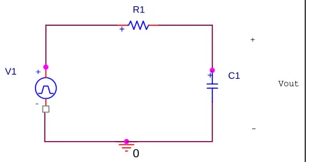
There is a basic need to be able to characterize a circuit independent of its circuit design and layout in order to predict its behavior. Consider the now-overly-familiar RC lowpass filter shown in Figure 1. We could describe this system by showing its circuit schematic or by calculating its impulse response or transfer function. But in many cases only FOMs are important to determine the adequacy of the system.

Figure 1. Simple RC lowpass filter circuit.

+

C1

Vout

-+

0 +

-V1

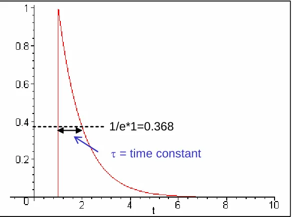
The first FOM is the system time constant. Many simple systems display a characteristic exponential decay (or rise) in their response. Since the form of the response is known, the only data important to characterize a specific system is the numerical value of its time constant. Figure 2 shows a typical impulse response for the RC filter of Figure 1. The characteristic exponential decay is just as we remember from class. The time constant of the circuit is defined as the time it takes for the response to decay to 1/e (37%) times its initial value. Since the functional form of the response is exp(-t/RC), the time constant of the circuit can easily be shown to be simply RC.

1/e*1=0.368

τ= time constant

1/e*1=0.368

τ= time constant

Figure 2. Impulse response of the RC lowpass filter circuit of Figure 1, showing the definition of the circuit time constant.

The time constant FOM allows us to determine the behavior of the circuit in a number of important scenarios, such as digital signal response or the time until steady-state analysis results are valid.

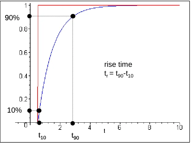
The second FOM, the risetime, characterizes the response of the system to a positive step change in input. The response of the circuit of Figure 1 to an applied unit step input is shown in Figure 3. The rise time most typically used as a FOM is the “10-90% risetime”, which is simply the amount of time necessary for the output to rise from 10% to 90% of its final value. This measurement in shown in Figure 3 as the time difference between the times t10 and t90. These

values can easily be determined given the step response of the system.

The 10-90% risetime FOM is especially important in digital systems, as excessive “slurring” of the crisp edges of the digital waveform leads to rapid degradation in system performance.

t₉₀ t10

rise time t_r= t₉₀-t₁₀ 90%

10%

t₉₀ t10

rise time t_r= t₉₀-t₁₀ 90%

10%

Figure 3. Step response of the RC lowpass filter circuit of Figure 1, showing the definition of the 10-90% risetime.

Measuring these two FOMs in the laboratory is actually a relatively simple effort for low bandwidth systems. The requirements are the circuit, or the system under test (CUT or SUT), and appropriate impulse and step waveform generation and measurement equipment. However, some thought needs to go into the waveform specification in order to facilitate measurement of the two FOMS.

The basic test setup is shown in Figure 4. The trick is to be able to create an “impulse” and a “unit step” waveform to test the system. Of course, we cannot create either of these two ideal waveforms in our part of the universe. However, we can create reasonable approximations.

function

generator scope

trigger trigger

Circuit FG output

input function

generator scope

trigger trigger

Circuit FG output

input

To simulate the impulse waveform, we could use a suitably abrupt and high amplitude pulse waveform. But what constitutes “suitably abrupt”? Well, if we can produce a pulse whose time width is much less than the time constant of the circuit, with a suitably large amplitude, then the pulse would provide a reasonable approximation of an impulse for that circuit. That same pulse might not be short enough in duration to approximate an impulse for a different circuit having a shorter time constant.

OK, now we see the trick. How can we approximate a unit step impulse? There are three important aspects of the step waveform to consider. First, the waveform must have a fast transition from off to on. Second, the waveform must stay “on” long enough for the system transients to die out. Thus, we could imagine a suitably wide pulse as being a reasonable approximation to a step input. The third aspect has to do with how we create the step change in the waveform.

Each of the two waveforms discussed above are single-shot events, or events that occur only once in time. The oscilloscopes we use are optimized for periodic waveforms, not single-shot events. No worries - we can create a pulse train with our function generators which allow for both control of pulse widths for impulse/step waveform design, as well as repeating these pulses periodically to optimize the viewing of the waveforms on the oscilloscope screen. However, the period of the waveform should be long enough to let all transients die out in the circuit before the next impulse arrives.

Pre-Lab Exercises

1. Calculate the impulse response of the RC lowpass filter shown in Figure 1, in terms of unspecified components R and C. Determine the time constant for the circuit.

2. Find the step response of the circuit, and determine the 10-90% rise time. . Specifically, show that the rise time is given by

r t

ln(9) r

t =τ

3. Specify values R and C which will produce a time constant of approximately 1 msec. Be sure to consider the fact that the capacitor will be asked to charge and discharge quickly in these measurements.

4. Show that the response of the circuit to a unit pulse of length T (, i.e. a pulse of amplitude 1 starting at 0 and ending at T) is given by

/ ( ) /

( ) (1 t ) ( ) (1 t T ) ( )

pulse

y t = −e− τ u t − −e− − τ u t T−

5. Plot the response to a unit pulse (Maple or Matlab) for τ =0.001 and , 0.001, and 0.0001 from 0 to 0.008 seconds. Note on the plots the times the capacitor is charging and discharging.

Equipment

Function Generator Oscilloscope

RC lowpass filter circuit of your design

Procedure

RC Circuit Impulse Response

1. Set up the laboratory equipment as shown in Figure 4. Be sure to use the higher

frequency capability function generator (why?). Record your equipment setup diagram. Construct your RC circuit using the values of R and C you determined in the Prelab exercises. Calculate the actual time constant for your circuit using actual measured component values.

2. Determine the waveform setting for the function generator shown in Figure 4 for simulating an impulse waveform for this circuit. Record these settings on the setup diagram in your notebook, and justify them. What is the area of your lab impulse?

3. Display the RC system impulse response on your oscilloscope screen and accurately sketch the input and output waveforms or place a plot showing both in your notebook. From the waveforms, determine the time constant for the circuit, and indicate it on the plot.

a. Compare the waveform and time constant you measured to your theoretical calculations from Step 1.

b. Compare the amplitude of your output exponential match to what you predicted in Step 2b.

Instructor Verification (see last page)

RC Circuit Step Response

4. Determine the waveform setting for the function generator shown in Figure 4 for simulating a step input waveform for this circuit. Record these settings on the setup diagram in your notebook, and justify them.

5. Display the RC system step response on your oscilloscope screen and accurately sketch the input and output waveforms or place a plot showing both in your notebook. From the waveform, determine the 10-90% rise time for the circuit and indicate it on the plot. Compare the waveform and risetime you measured to your theoretical calculations.

Instructor Verification (see last page)

Report

Record the results of all of your work in one partner’s lab notebook. Tape any printout (graphs, for example) into the notebook as specified in the Lab Manual for the course. (You must provide your own tape.) Be sure that all members of your lab group sign the lab notebook, and hand the notebook in at the end of lab.

System Impulse and Step Response

Instructor Verification Sheet

Turn this page in to your Professor

Name ___________________________________________ Date of Lab: __________________

Part (3) Display impulse response and compare RC time constant measurement with calculation.

Verified: _________________________________________ Date/Time: __________________

Part (5) Display step response and compare with theory.