Scalable Machine Learning Methods for Massive Biomedical Data Analysis.

(1)

Scalable Machine Learning Methods for

Massive Biomedical Data Analysis

by

Takanori Watanabe

A dissertation submitted in partial fulfillment of the requirements for the degree of

Doctor of Philosophy (Electrical Engineering: Systems)

in The University of Michigan 2015

Doctoral Committee:

Associate Professor Clayton D. Scott, Co-Chair Assistant Professor Chandra S. Sripada, Co-Chair Professor Jeffrey A. Fessler

Professor Alfred O. Hero III Professor Charles R. Meyer

(2)

c

(3)

(4)

LIST OF FIGURES

Figure

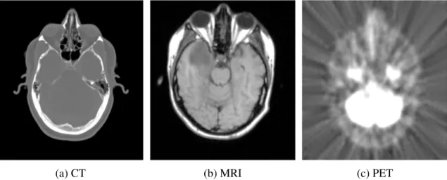
1.1 Example execution of the registration process. . . 5 1.2 Brain images acquired from different imaging modalities. Note the

variation in the appearance of the anatomy. . . 6 1.3 The impact of the choice of similarity measureΨ. Top row: successful

intramodal registration using SSD.Middle row: unsuccessful intermodal registration using SSD; note the misalignment in the corpus callosum, which has a black appearance in the reference image and a white appearance in the homologous image. Bottom row: successful intermodal registration using mutual information. . . 7 2.1 Conceptual illustration of the proposed method. The marks in (a)-(b) are

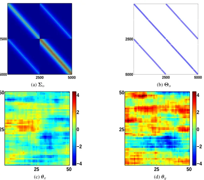
a few point-correspondences estimated by registration. The confidence regions in (c) offer an understanding of the possible registration error for these pixels. We expect the shape of the confidence regions to reflect the local image structure, as demonstrated in (c). . . 18 2.2 Illustration of the properties of the baseline covarianceΣo. The values

used are pnx, nyq p50,50q, prx, ryq p0.95,0.8q, andtcx, cy, cxyu

t1,2,0.5u. (a) The baseline covarianceΣo, (b) the sparsity structure of Θo Σo1, (c)-(d) B-spline coefficientsθx andθy obtained from sample θ pθx,θyq Np0,Σoq. . . 23 2.3 The top two rows show the2-D dataset used in the first experiment, along

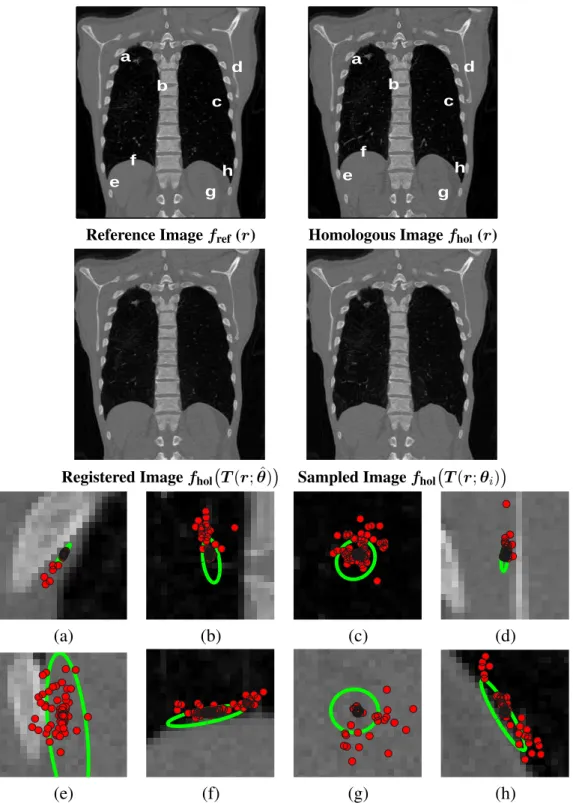
with the registration result and an image synthesized using one of the sampled deformations. A few of the confidence regions from r P Ωref are shown in (a)-(h), with the red marks representing100 realizations of registration error. Note how the confidence regions reflect the local image structure. . . 28

(8)

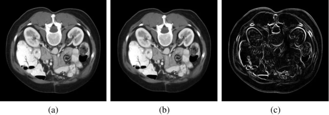
2.4 The dataset used for validation: (a) the homologous imagef_holprq, (b) the reference imagefrefprq fhol Tpr;θq

generated by a deformation coefficient sampled from the ground-truth distributionθ Npµθ,Σθq,

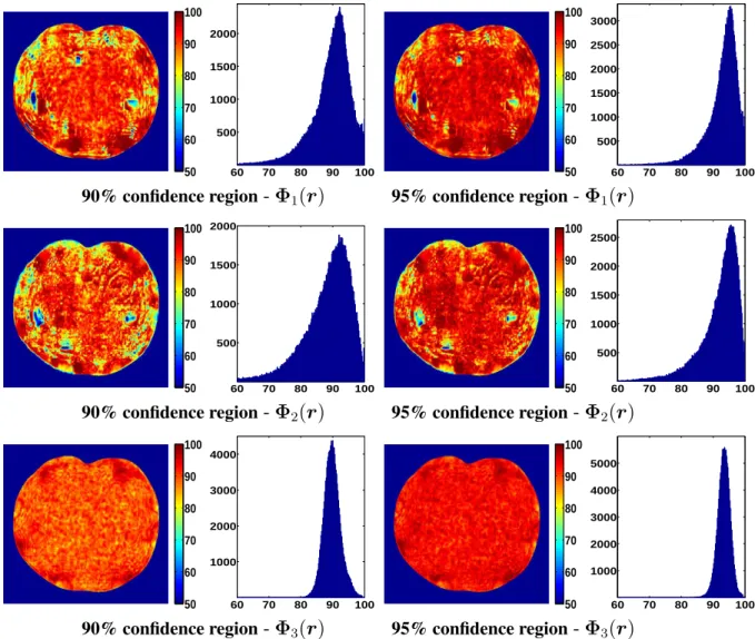
(c) the absolute difference image. . . 29 2.5 The coverage rates evaluated for the three classes of spatial confidence

regions presented in Table 2.1, displayed in the form of heatmap and histogram. Note that the performances of Φ1prq and Φ2prq are fairly

comparable to the ideal confidence region Φ3prq, as the coverage rates

for many of the pixels come close to the prespecified confidence levelγ. . 31 3.1 Coronal, sagittal, and axial slices depicting the coverage of our brain

parcellation scheme along with3-D rendering of one pseudo-sphereical node. Each contiguous green region represents a pseudo-spherical node representing an ROI containing 33-voxels. Overall, there are 347 non-overlapping nodes placed throughout the entire brain. These nodes are placed on a grid with18mm spacing between node centers in theX, Y, andZ dimensions. . . 39 3.2 Illustration of the neighborhood structure of the connectome when the

nodes reside in 2-D space. The red edge represents coordinate j

p2,4q,p6,2q( in 4-D connectome space, and its neighborhood set Nj is represented by the blue and green edges. This idea extends directly to 6-D connectomes generated from3-D resting state volumes. . . 45 3.3 Laplacian matrix corresponding to the original data CT_C _{and the}

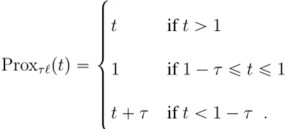
augmented data CrTC, where the rows and columns of these matricesr represent the coordinates of the original and augmented functional connectome. Note that the irregularities in the original Laplacian matrix are rectified by data augmentation. The augmented Laplacian matrix has a special structure known as block-circulant with circulant-blocks (BCCB), which has important computational advantages that will be exploited in this work. . . 49 3.4 Plots of scalar convex loss functions that are relevant in this work, along

with their associated proximal operators. Table3.1 provides the closed form expression for these functions. Parameter values of τ 2 and δ 0.5are used in the plot for the proximal operator and the huberized hinge-loss respectively. . . 55

(9)

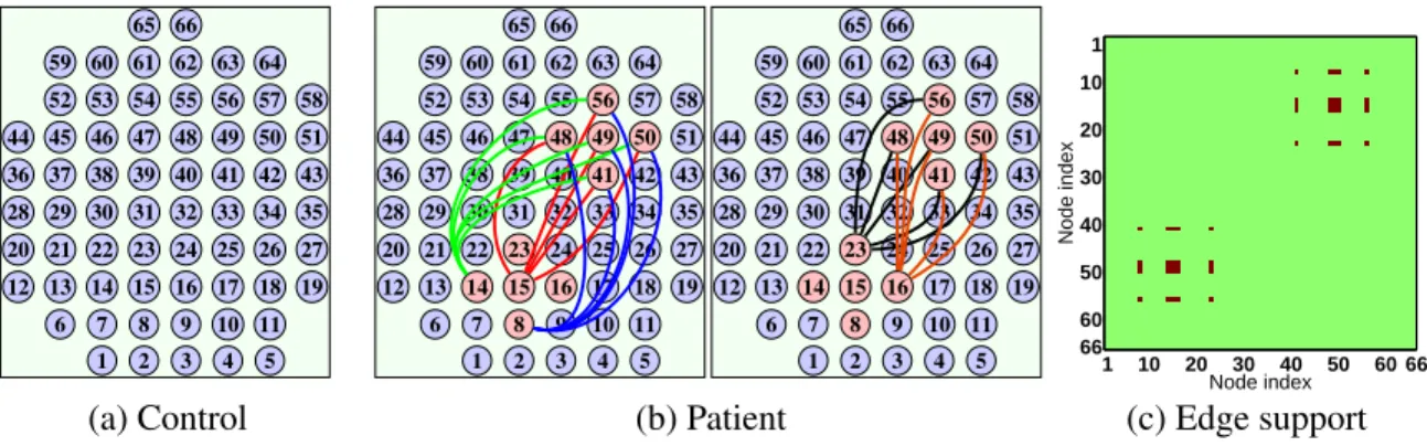
3.5 Schematic representations of the synthetic 4-D functional connectome data generated for the simulation experiments (best viewed in color). (a) Node orientation representing the “control class” connectome, where the blue nodes indicate the normal nodes. (b) Node orientation representing the “patient class” connectome, where there are 25 anomalous edges shared among the two anomalous node clusters indicated in red (this subfigure is split into two side-by-side figures to improve visibility of the impacted edges). (c) Binary support matrix indicating the locations of the anomalous edges in the connectome space. . . 60 3.6 Simulation experiment result: training set consists ofn 100 samples

with 50patients and 50 controls (best viewed in color). (a)-(d) Weight vectors (reshaped into symmetric matrices) estimated from solving the regularized ERM problem (3.1) using the hinge-loss and four different regularizers. Regularization parameters were tuned via 5-fold cross-validation on the training set, and classification accuracies were evaluated on a testing set consisting of 500 samples with 250 patients and 250 controls. (e) Support matrix indicating the locations of the anomalous edges. (f) ROC curve representing the anomalous edge identification accuracy (not classification accuracy) of the four regularizers. . . 66 3.7 Grid search result for the simulation experiment (best viewed in color).

All classifiers were learned using 100 training samples consisting of 50 patients and 50 controls. Top two rows: classification accuracy as a function of the regularization parameters tλ, γu (evaluated from 500 testing samples consisting of250patients and250controls). Bottom two rows: the number of features selected as a function of the regularization parameterstλ, γu. . . 68 3.8 The testing classification accuracy of the different regularizers as a

function as a number of training samplesnin the simulation experiment. Regularization parameters were tuned via5-fold cross-validation on the training set. The testing set consists of500samples with250patients and 250controls. Table3.3reports the actual numbers. . . 69 3.9 Grid search result for the real resting state data (best viewed in color).

Top row: the classification accuracy evaluated from 10-fold cross-validation. Bottom row: the average number of features selected across the cross-validation folds. Thepx, yq-axis corresponds to the two regularization parametersλandγ. . . 71

(10)

3.10 Weight vectors (reshaped into symmetric matrices) generated by computing the elementwise median of the estimated weight vectors across the cross-validation folds (best viewed in color). The rows and columns of these matrices are grouped according to the network parcellation scheme proposed by Yeo et al. (2011), which is reported in Table 3.4. The top row displays the heatmap of the estimated weight vectors, whereas the bottom row displays their support structures, with red, blue, and white indicating positive, negative, and zero entries respectively. In order to highlight the structure of the estimated weight vectors, the bottom row further plots the degree of the nodes, i.e., the number of connections a node makes with the rest of the network. . . 73 3.11 Nonzero edge values of the median weight vector generated from

the fused Lasso regularized SVM. For three sets of network-to-network connections, we rendered abnormal connections separately on anterior, sagittal, and axial views of a canonical brain. Notice the prominent involvement of lateral prefrontal regions in connections within frontoparietal network and in connections between frontoparietal network and default network. . . 75 3.12 The effect of the first level augmentation matrixA1. Left: the original

functional connectomexonly contains edges between the nodes placed on the support of the brain (represented by the green nodes). Right: A1 pads extra zero entries on x to create the intermediate augmented

connectome x. Here, x can be treated as if the nodes were placed throughout the entire rectangular FOV (the red bubbles represent nodes that are outside the brain support), as its entries contain all possible edges between the green and red nodes; the edges that connect with the red nodes all have zero values. . . 89 3.13 The effect of the second level augmentation matrixA2. The entries of

xrepresent edges localized by6-D coordinate pointstprj,rkq |j ¡ku, whererj pxj, yj, zjqandrk pxk, yk, zkqare the3-D locations of the node pairs defining the edges. A2 fixes the asymmetry in the coordinates

of x by padding zero entries to accommodate for the 6-D coordinate pointstprj,rkq |j ¤ku; these are the diagonal and the upper-triangular entries in the cross-correlation matrix that were disposed for redundancy. 89 4.1 Sagittal, coronal, and axial slices depicting the coverage of our brain

parcellation scheme, where each nodes represents an ROI encompassing 33-voxels. Overall, there are 347 non-overlapping nodes placed throughout the entire brain. These nodes are placed on a grid with 18 mm spacing between node centers in theX, Y, andZ dimensions. The color of the nodes represents the network membership according to the parcellation scheme proposed byYeo et al.(2011), as outlined in (d). . . 97

(11)

4.2 Comparison between the sparsity patterns promoted by the single-task `1{`1 and the multitask `1{`2 penalty. The rows in the matrices above

represent the task-specific weight vectors wk(K_k₁, and the blue entries indicate the non-zero coefficients. Note how the single-task approach yields sparsity patterns that are inconsistent across sites, which can be problematic for interpretation. In contrast, thegroup variable selection property from the multitask approach provides a sparsity pattern that is shared across all sites. . . 103 4.3 The ROC curves obtained by varying the threshold of the classifiers in

Table 4.3 classifiers’ ROC. The ROC curves for the single-task `1{`1

-case are omitted to improve curve visibility. (EN = Elastic-net, GN = GraphNet, FL = fused Lasso, TV = isotropic total variation). . . 114 4.4 Classification accuracy evaluated from 5-fold cross-validation (best

viewed in color). The px, yq-axis corresponds to the two regularization parametersλandγ. . . 116 4.5 Average number of features selected across the cross-validation folds

(best viewed in color). The px, yq-axis corresponds to the two regularization parametersλandγ. . . 117 4.6 Weight vectors estimated from the Elastic-net+`1{`2 and fused

Lasso+`1{`2-penalized SVM. Left: support matrices of the selected

features (rows/cols grouped by network membership).Right:brain space representation of the selected edges in the intra-frontoparietal (6-6: blue) and the intra-default network (7-7: red). . . 118

(12)

LIST OF TABLES

Table

2.1 Spatial Confidence Regions Generated for Validation . . . 29 3.1 Examples of scalar convex loss functions that are relevant for this work,

along with their corresponding proximal operators in closed form. . . 55 3.2 Demographic characteristics of the participants before and after sample

exclusion criteria is applied (RH = right-handed). . . 62 3.3 The testing classification accuracy of the different regularizers as a

function as a number of training samplesn in the simulation experiment (the best classification accuracy for eachn is denoted in bold font). See Fig.3.8for a plot of this result. . . 69 3.4 Network parcellation of the brain proposed byYeo et al. (2011). In our

real resting state fMRI study, the indices of the estimated weight vectors are grouped according to this parcellation scheme; see Fig.3.10. . . 73 4.1 Sample characteristics of the participants in the training set, shown both

before and after application of exclusion and quality control criteria. Acronyms are: KKI = Kennedy Krieger Institute, NYU = New York University, OHSU = Oregon Health and Science University, Wash. U = Washington University in St. Louis. . . 94 4.2 Sample characteristics of the participants in the validation test set, shown

both before and after application of exclusion and quality control criteria. 95 4.3 The classification results from the 5-fold cross-validation and the

validation test-set. . . 113 4.4 Network parcellation scheme of the brain proposed byYeo et al.(2011). . 118

(13)

ABSTRACT

Scalable Machine Learning Methods for Massive Biomedical Data Analysis by

Takanori Watanabe

Chair: Clayton D. Scott Co-chair: Chandra S. Sripada

Modern data acquisition techniques have enabled biomedical researchers to collect and analyze datasets of substantial size and complexity. The massive size of these datasets allows us to comprehensively study the biological system of interest at an unprecedented level of detail, which may lead to the discovery of clinically relevant biomarkers. Nonetheless, the dimensionality of these datasets presents critical computational and statistical challenges, as traditional statistical methods break down when the number of predictors dominates the number of observations, a setting frequently encountered in biomedical data analysis. This difficulty is compounded by the fact that biological data tend to be noisy and often possess complex correlation patterns among the predictors. The central goal of this dissertation is to develop a computationally tractable machine learning framework that allows us to extract scientifically meaningful information from these massive and highly complex biomedical datasets. We motivate the scope of our study by considering two important problems with clinical relevance: (1) uncertainty analysis for biomedicalimage registration, and (2) psychiatric disease prediction based on functional

(14)

connectomes, which are high dimensional correlation maps generated from resting state functional MRI.

The first part of the dissertation concerns the problem of analyzing the level of uncertainty involved in biomedical image registration, where image registration is the process of finding the spatial transformation that best aligns the coordinates of an image pair. Toward this end, we introduce a data-driven method that allows one to visualize and quantify image registration uncertainty using spatially adaptive confidence regions, and demonstrate that empirical evaluations of the method on2-D images yield promising results. At the heart of our proposed method is a novel shrinkage-based estimate of the distribution on deformation parameters.

The second part of the dissertation focuses on the supervised learning problem of binary classification, where the goal is to predict the psychiatric disorder status of an individual using functional connectomes derived from resting-state functional MRI. To address the dimensionality of the features, we introduce a regularized empirical risk minimization framework that allows us to encode various structures in the data. Specifically, in contrast to previous methods, our approach explicitly accounts for the 6-D spatial structure of the functional connectomes (defined by pairs of points in 3-D space) by using either the GraphNet, fused Lasso, or the isotropic total variation penalty. Furthermore, we also introduce a multitask extension to this framework, which is suitable when the data are aggregated from multiple imaging institutions. Experiments on both synthetic and real world data reveal that the proposed method can recover results that are more neuroscientifically informative than previous methods while improving predictive performance.

(15)

CHAPTER 1

Introduction

With advancing data acquisition technology, high dimensional data have become much more regularly encountered in various areas of biomedical science. For example, advanced microarray technology allows scientists to measure the expression levels of tens of thousands of genes in a single experiment. In addition, modern neuroimaging techniques afford a variety of modalities that produce large-scale measurements that represent different aspects of neuronal activity, such as functional magnetic resonance imaging (fMRI), positron emission tomography (PET), and electroencephalograms (EEG) and magnetoencephalograms (MEG) recordings. The massive size of these data offers new possibilities, as they allow us to comprehensively study the biological system of interest at an unprecedented level of detail, which may lead to the discovery of clinically relevant biomarkers1_. _{Nonetheless, the dimensionality of these data presents critical}

computational and statistical challenges, as traditional statistical methods break down when the number of parameters (predictors) dominates the number of observations, a setting frequently encountered in biomedical data analysis. This difficulty is compounded by the fact that biological data often possess complex correlation patterns among the predictors and tend to be noisy for variety of reasons, such as background noise, calibration error in

1_{The word} _biomarker _{is formally defined by the National Institutes of Health Biomarkers Definitions}

Working Group as: “a characteristic that is objectively measured and evaluated as an indicator of normal biological processes, pathogenic processes, or pharmacologic responses to a therapeutic intervention” (Atkinson et al.,2001;Strimbu and Tavel,2010).

(16)

the measurement device, physiological movements (e.g., cardiac and respiratory motion), and other sources of experimental variations. The central goal of this dissertation is to develop a computationally tractable machine learning framework that allows us to extract scientifically meaningful information from these massive and highly complex biomedical data. We motivate the scope of our study by considering two important problems with clinical relevance: (1) uncertainty analysis for biomedical image registration, and (2) psychiatric disease prediction based on functional connectomes, which are high dimensional correlation maps generated from resting state fMRI.

The remainder of this introductory chapter is organized as follows. First, we will formally present the challenges encountered in high dimensional data analysis, and introduce some of the key tools we utilize to mitigate these problems. Next, we will provide a brief primer on image registrationandfunctional connectomes, and present the main contributions of our work. Finally, we will conclude this chapter with an outline of the dissertation.

1.1 High Dimensional Challenges

The setup where the number of parameters p greatly exceeds the sample size n is commonly referred to as the “large p small n problem,” denoted p " n (Bühlmann and van de Geer, 2011; West, 2003). In such setting, classical statistical methods break down in the face of the “curse of dimensionality” (Donoho, 2000; Duda et al., 2000). More concretely, the estimation procedure becomes susceptible to overfitting, i.e., the estimated model will perform extremely well on the training data, but will predict poorly on unobserved data. Furthermore, in the p " n setup, it is impossible to attain a statistically consistent estimator unless we impose some type of structural assumption on the model (Negahban et al.,2012). This leads us to the notion ofregularization, a concept that will appear throughout this dissertation.

(17)

Tikhonov, 1963), and is achieved by encoding prior knowledge about the data structure into the estimation problem. In fact, many well known estimators from statistics and machine learning are based on solving aregularized empirical risk minimizationproblem (e.g., support vector machine, logistic regression, boosting) that has the following form:

arg min

wPRp

Lpwq λRpwq. (1.1)

The first termL : _Rp _Ñ

R corresponds to theempirical risk of some loss function (e.g.,

square loss, Huber loss, hinge loss), which quantifies how well the model fits the data. The second termR:_Rp Ñ

R is aregularizer that curtails overfitting and enforces some kind

of structure on the solution by penalizing models that deviate from the assumed structure. The user defined regularization parameter λ ¥ 0 controls the tradeoff between data fit and regularization. Several different regularizers have been proposed in the literature to promote various forms of structure, such as smoothness (e.g., ridge regression (Hoerl and Kennard, 1970), support vector machine (Cortes and Vapnik,1995)), sparsity (e.g., Lasso (Tibshirani, 1996), basis pursuit (Chen et al., 2001)), group sparsity (e.g., group Lasso (Yuan and Lin,2006), latent group Lasso (Obozinski et al.,2011)), low-rank structure (e.g., trace/nuclear norm (Bach, 2008b; Recht et al., 2010)), and sparse covariance and inverse covariance structure (Bien and Tibshirani, 2011;Friedman et al., 2007;Meinshausen and Bühlmann,2006).

Finally, an equally important aspect of a learning method is its computational tractability, as many statistical learning problems involve solving a numerical optimization problem (e.g., Equation1.1). In principle, almost all convex optimization problems can be solved with high accuracy using polynomial time interior-point methods. However, these generic solvers are impractical for high dimensional data, since the iteration cost of these methods grows nonlinearly with the problem sizep(Boyd and Vandenberghe,2004;

(18)

Elastic-net), which are commonly used in high dimensional statistical inference problems, add to the difficulty by introducing non-differentiability to the objective function. For this reason, first-order optimization methods have generated renewed interest from the statistics and machine learning community, as they are capable of solving large scale and often nonsmooth optimization problems. These methods include conjugate gradient, proximal gradient, projected gradient, and alternating direction methods (Bach et al.,2012;Beck and Teboulle,2009;Boyd et al.,2011;Nesterov,2007). The work presented in the dissertation will frequently rely on these types of first-order optimization techniques.

1.2 Biomedical Image Registration and Uncertainty Analysis

Image registration is the process of finding the spatial transformation that maps the homologous image’s coordinate space to the reference image’s coordinates; Fig. 1.1

provides an example execution of the registration process. Its ability to fuse medical images with complementary information has led to its adoption in a variety of clinical research settings (Hill et al., 2001). For instance, PET and MRI are modalities that are commonly used for surgical planning. On one hand, PET images contain information about cancerous activity within the brain, but do not contain much anatomical structure. On the other hand, MRI images capture anatomical structures in the brain, but provide little physiological information. The variation in the appearance of the anatomy from these modalities can be seen in Fig.1.2. By registering these images, the cancerous anatomical structures can be localized in a unified coordinate system. Other medical applications of image registration include motion correction, atlas construction, dose estimation, treatment monitoring, radiation therapy, and many more (Hill et al.,2001;Long et al.,2010;Shi et al.,

(19)

1.2.1 Background: Elements of Biomedical Image Registration

Image registration is typically cast as an optimization problem, where the goal is to find the transformation that optimizes a user specified similarity measure that quantifies the quality of alignment between the reference image and the transformed homologous image. More formally, given a pair ofd-dimensional imagesfref andfhol, image registration aims to solve the following optimization problem:

ˆ T arg max T Ψ frefpq,fholTpq , (1.2)

where fref : Rd Ñ R and fhol : Rd Ñ R are the reference and the homologous image respectively,T :_RdÑ_Rddenotes the spatial transformation that models the misaligment between the image pair, and Ψ is a user-specified similarity measure that quantifies the quality of the alignment. Importantly, Equation 1.2 illustrates the following three major design components of image registration:

1. the similarity measureΨ,

2. the model for the spatial transformationT,

3. the optimization algorithm for solving (1.2).

(a) Reference image (b) Homologous image (c) Registered image

(20)

(a) CT (b) MRI (c) PET

Figure 1.2: Brain images acquired from different imaging modalities. Note the variation in the appearance of the anatomy.

Similarity measure (Ψ): The choice of the similarity measure depends on the type of relationship one expects among the pixel (voxel) intensities in the image pair. For example, in the intramodal setup, where the images are acquired from the same imaging modality, it is reasonable to assume the intensities of the images to be directly/linearly related. Thus simple similarity measures such as the sum of squared differences (SSD) and Pearson’s correlationare popular choices for this setup. Conversely, in theintermodalsetup, where the images are acquired from different imaging modalities, the intensities of the two images are no longer directly related, hence SSD and Pearson’s correlation become inappropriate. In this case, usually one instead assumes a statistical/probabilistic relationship between the images, and information theoretic measures such as conditional entropy and mutual informationare common choices (Pluim et al.,2003). Fig.1.3illustrates how the choice of the similarity measure can have a huge impact on the outcome of a registration algorithm.

Transformation model (T): The transformation model describes the type of spatial deformation that is expected between the reference and the homologous image. A parametric approach is commonly adopted for this, where the transformation T is compactly characterized by a parameter vector θ; the size of θ determines the degrees of freedom (DOF) of the model. The simplest choice is the rigid transformation model

(21)

(a) Reference (b) Homologous (c) Registered homologous Figure 1.3: The impact of the choice of similarity measure Ψ. Top row: successful intramodal registration using SSD.Middle row: unsuccessful intermodal registration using SSD; note the misalignment in the corpus callosum, which has a black appearance in the reference image and a white appearance in the homologous image. Bottom row: successful intermodal registration using mutual information.

(22)

that is characterized by rotation and translation, corresponding to three DOF in 2-D and six DOF in 3-D. While this model is appropriate for describing movements in the hard tissue region, it is not capable of capturing local movements in the soft tissue area (e.g., respiratory and cardiac motion). To model these types of local deformations, nonrigid transformation models such as the B-spline and thin-plate spline models are commonly used (Meyer et al., 1997; Rueckert et al., 1999; Unser, 1999). Extensive reviews on nonrigid deformation models can be found in (Holden,2008;Sotiras et al.,2013). However, the flexibility afforded by the nonrigid model comes at the expense of the size of the parameter vector θ, which can often be on the order of a million. This not only increases computational complexity but also leads to overfitting, which results in a physically unrealistic transformation such as bone-warping. Thus, regularization becomes crucial for stabilizing the estimation procedure, and various regularizers have been introduced in the literature, such as the gradient norm, elastic energy, topology preserving penalty (Chun and Fessler,2009;Modersitzki,2004)).

Optimization strategies: As explained earlier, image registration is an optimization problem that aims to find the transformation that best aligns the coordinates of an image pair. Hence the choice of the optimization strategy can have a significant impact on the outcome of the registration algorithm. Iterative gradient based approaches such as gradient descent, conjugate gradient descent, and quasi-Newton methods are frequently used for nonrigid models with high DOF (Holden,2008;Klein et al.,2007;Sotiras et al.,2013).

(23)

1.2.2 Contribution: Registration Uncertainty Analysis using Spatial Confidence Regions

Despite the promises that image registration offers, there are numerous issues that still must be solved before it can be used in the clinical practice. For instance, it is well known that registration accuracy is limited in practice, and the degree of uncertainty varies at different image regions. Such uncertainty arises for variety of reasons, such as the variation in the appearance of the anatomy, measurement noises, deformation model mismatch, local minima, etc. Evaluating this degree of uncertainty is highly non-trivial due to the scarcity of ground-truth data. Understanding the accuracy of a registration result is one of the central themes in modern medical image analysis.

In light of these challenges, in Chapter 2 of the dissertation, we propose a data-driven method that allows one to visualize and quantify the registration uncertainty through spatially adaptive confidence regions. The method applies to any choice of the similarity measure and various parametric transformation models, including high dimensional deformation models such as the B-spline. At the heart of the proposed method is a novel shrinkage-based estimate of the distribution on deformation parameters θ. We present some empirical evaluations of the method in2-D using images of the lung and liver, and demonstrate that the confidence regions produces promising results.

1.3 Disease Prediction based on Functional Connectomes

The emerging field of connectomics, which is the study of the network architecture of the brain, has provided various new insights about neuropsychiatric disorders that are associated with abnormalities in brain connectivity (Biswal et al., 2010; Hagmann, 2005;

Sporns et al., 2005). Brain connectivity can be broadly divided into two categories: structural connectivity and functional connectivity. On one hand, “structural connectivity” describes anatomical connections, i.e., physical wiring of the brain such as linkages

(24)

in white matter fiber tracts that can be studied using modalities such as diffusion tensor images (DTI) (Bihan and Johansen-Berg, 2012). On the other hand, “functional connectivity” describes functional connections that are typically characterized by the statistical dependencies among the neuronal signals between remote brain regions (Biswal et al., 1995). These brain connectivities are commonly represented as graphs called structural and functional connectomes, where the nodes represent brain regions and the edges (weighted or binary) represent the structural/functional relationship between the neuronal signals (Bullmore and Sporns, 2009; Smith et al., 2013; Sporns, 2013). Throughout this dissertation, we will focus on functional connectomes generated from resting statefMRI.

1.3.1 Background: Resting state fMRI and Functional Connectomes

FMRI data consist of a time series of three dimensional volumes imaging the brain, where each3-D volume encompasses around10,000100,000voxels. The univariate time series at each voxel represents a blood oxygen level dependent (BOLD) signal, an indirect measure of neuronal activities in the brain. The imaging process is noninvasive, relatively cheap and accessible, and does not expose subjects to radiation, making fMRI an attractive tool for studying the human brain.

Traditional experiments in the early years of fMRI research involvedtask-based studies, where participants perform a set of tasks during scan time, and the goal is to identify the brain regions associated with the task performance. However, it was later discovered that even in the absence of a cognitive task performance, the BOLD signal follows a synchronized fluctuation pattern at distributed brain regions (Biswal et al.,1995), implying that the brain is functionally connected at rest (Greicius et al., 2003). These temporal correlations between remote brain regions is referred to asfunctional connectivity(Friston,

1994), and resting state fMRI has become a vital modality for studying the intrinsic functional architecture of brain networks (Fox and Raichle,2007;Smith et al.,2013).

(25)

A particularly notable tool that made a significant contribution in the development of the field of connectomics isfunctional connectome, which is a correlation map derived from resting state fMRI. More precisely, functional connectomes are constructed by parcellating the brain into multiple distinct regions and computing cross-correlations among the inter-regional BOLD signals (Varoquaux and Craddock,2013). It is important to note that even with a relatively coarse parcellation scheme with several hundred regions of interest (ROI), the resulting functional connectome will be massive, encompassing hundreds of thousands of connections or more.

A central goal in connectomic research is the identification of an objective, connectivity-based biomarker of psychiatric disorders using functional connectomes. Such discovery would not only substantially extend our knowledge about the network topology of the human brain, but also offers the potential for a machine-based diagnosis system to enter the clinical realm (Atluri et al., 2013). Thus in recent years, machine learning techniques have garnered considerable amount of interests among the neuroimaging community (Pereira et al., 2009; Richiardi et al., 2013). However, many standard “off-the-shelf” machine learning algorithms are not immediately applicable due to the massive size of functional connectomes. Thus, a specialized class of machine learning techniques that are amenable to the dimensionality of functional connectomes is in critical need.

1.3.2 Contribution: Connectome-based Disease Prediction using a Scalable and Spatially-Informed Support Vector Machine

Abundant neurophysiological evidences indicate that major psychiatric disorders such as Alzheimer’s disease, Attention Deficit Hyperactive Disorder (ADHD), autism spectrum disorder (ASD), and schizophrenia are associated with altered connectivity in the brain (Bassett and Bullmore, 2009; Castellanos et al., 2013; Dey et al., 2012; Fornito et al.,

2012; Fox and Greicius, 2010; Sripada et al., 2014). Thus, there is great interest in developing machine-based methods that reliably distinguish patients from healthy controls

(26)

using neuroimaging data. In this dissertation, we are specifically interested in a multivariate approach that uses features derived from whole-brain resting state functional connectomes. However, functional connectomes reside in a high dimensional space, which complicates model interpretation and introduces numerous statistical and computational challenges. Traditional feature selection techniques are used to reduce data dimensionality, but are blind to the spatial structure of the connectomes (Castellanos et al.,2013;Craddock et al.,

2009;Dai et al.,2012;Sripada et al.,2013b;Zeng et al.,2012).

In Chapter 3, we address these issues by proposing a regularization framework where the6-D structure of the functional connectome (defined by pairs of points in 3-D space) is explicitly taken into account via the sparse fused Lasso (Tibshirani et al., 2005) or the GraphNet regularizer (Grosenick et al., 2013). Our method only restricts the loss function to be convex and margin-based, allowing non-differentiable loss such as the hinge-loss to be used. Using the fused Lasso or GraphNet regularizer with the hinge-loss leads to a structured sparse support vector machine (SVM) with embedded feature selection. We introduce a novel efficient optimization algorithm based on augmented Lagrangian and the classical alternating direction method (Boyd et al.,2011), which can solve both fused Lasso and GraphNet regularized SVM with very little modification. We also demonstrate that the inner subproblems of the algorithm can be solved efficiently in analytic form by coupling the variable splitting strategy with a data augmentation scheme. Experiments on simulated data and resting state scans from a large schizophrenia dataset show that our proposed approach can identify predictive regions that are spatially contiguous in the 6-D “connectome space,” offering an additional layer of interpretability that could provide new insights about various disease processes.

(27)

1.3.3 Contribution: Multitask Structured Sparse Support Vector Machine for Multisite Connectivity-based Disease Prediction

In response to the significant interest in developing imaging-based methods for diagnosing neuropsychiatric conditions, several data-sharing initiatives have been launched in the neuroimaging field (Biswal et al., 2010;Di Martino et al., 2013;Essen et al.,2012;

Mennes et al.,2013;Poldrack et al.,2013;Poline et al.,2012;The ADHD-200 Consortium,

2012; Weiner et al., 2012). Here the datasets are collected across multiple imaging sites throughout the world. While this enables researchers to study the disorders of interest with substantial sample size, it also creates new challenges since the data aggregation process introduces various sources of site-specific heterogeneities.

To address this issue, in Chapter 4 we introduce a multitask structured sparse SVM, an extension to the method introduced in Chapter 3. Specifically, we employ a penalty that accounts for the following two-way structure that exists in a multisite functional connectome dataset: (1) the6-Dspatial structurein the functional connectomes captured via either the GraphNet, fused Lasso, or the isotropic total variation penalty, and (2) the inter-sitestructure captured via the multitask`1{`2-penalty (Lounici et al.,2009;Obozinski

et al.,2010). The potential utility of the proposed method is demonstrated on the multisite ADHD-200 dataset.

1.4 Dissertation Outline

The remainder of the dissertation is organized as follows. In Chapter 2, we introduce a novel data-driven method that allows one to visualize and quantify image registration uncertainty using spatially adaptive confidence regions. In Chapter 3, we present a statistical learning framework for predicting the neuropsychiatric disease status of an individual usingfunctional connectomes generated from resting state fMRI. In contrast to previous approaches, the method we present explicitly accounts for the6-D spatial structure

(28)

of the data. Chapter4presents a multitask extension to the work of Chapter3, where the imaging sites are treated as the tasks. Finally, we conclude in Chapter 5 by providing a summary of the dissertation, and outline directions for future work.

(29)

CHAPTER 2

Spatial Confidence Regions for Quantifying and

Visualizing Registration Uncertainty

For image registration to be most useful in a clinical setting, it is desirable to know the degree of uncertainty in the returned point-correspondences. In this chapter, we propose a data-driven method that allows one to visualize and quantify the registration uncertainty through spatially adaptive confidence regions. The method applies to any parametric deformation models and to any choice of the similarity criterion. We adopt the B-spline model and the negative sum of squared differences for concreteness. At the heart of the proposed method is a novel shrinkage-based estimate of the distribution on deformation parameters. We present some empirical evaluations of the method in2-D using images of the lung and liver, and the method generalizes to3-D.

2.1 Introduction

Image registration is the process of finding the spatial transformation that best aligns the coordinates of an image pair. Its ability to combine physiological and anatomical information has led to its adoption in a variety of clinical settings. However, the registration process is complicated by several factors, such as the variation in the appearance of the

(30)

anatomy, measurement noises, deformation model mismatch, local minima, etc. Thus, registration accuracy is limited in practice, and the degree of uncertainty varies at different image regions. For image registration to be most useful in clinical practice, it is important to understand its associated uncertainty.

Unfortunately, evaluating the accuracy of a registration result is non-trivial, mainly due to the scarcity of ground-truth data. For rigid-registration, there have been studies where physical landmarks are used to perform error analysis (Fitzpatrick and West,2001). Statistical performance bounds for simple transformation models have been presented under a Gaussian noise condition (Robinson and Milanfar, 2004; Yetik and Nehorai,

2006). However, it is generally difficult or impractical to extend these methods to nonrigid registration, which limits their applicability since many part of the human anatomy cannot be described by a rigid model.

While characterizing the accuracy of a nonrigid registration algorithm is even more challenging, there have been recent works addressing this issue. Christensen et al.(2006) initiated a project which aims to allow researchers to perform comparative evaluation of nonrigid registration algorithms on brain images. Ruan and Fessler(2008) presented an observation model for image registration that accounts for image noise, and analyzed the performance limit of the model using Cramér-Rao bound analysis. Kybic (2010) used bootstrap resampling to perform multiple registrations on each bootstrap sample, and used the results to compute the statistics of the deformation parameter. Hub et al. (2009) proposed an algorithm and a heuristic measure of local uncertainty to evaluate the fidelity of the registration result. Risholmet al. adopted a Bayesian framework in (Risholm et al.,

2010), where they proposed a registration uncertainty map based on the inter-quartile range (IQR) of the posterior distribution of the deformation field. Simpsonet al. also adopted the Bayesian paradigm in (Simpson et al., 2012), where they introduced a probabilistic model that allows inference to take place on both the regularization level and the posterior of the deformation parameters. The mean-field variational Bayesian method was used to

(31)

approximate the posterior of the deformation parameters, providing an efficient inference scheme.

We view the deformation as a random variable and propose a method that estimates the distribution of the deformation parameters given an image pair and registration algorithm. For illustration purpose, we use the cubic B-spline deformation model and the negative sum of squared differences as the similarity criterion, but the idea is applicable for other forms of parametric model (see Holden (2008) for other possible choices) and intensity-based registration algorithms. The estimated distribution will allow us to simulate realizations of registration errors, which can be used to learn spatial confidence regions. To the best of our knowledge, none of the existing methods view the registration uncertainty through spatial confidence regions represented in the pixel-domain. The confidence regions can be used to create an interactive visual interface that can be used to assess the accuracy of the original registration result. A conceptual depiction of this visual interface is shown in Fig. 2.1. When a user, such as a radiologist, selects a pixel in the reference image, a confidence region appears around the estimated corresponding pixel in the homologous image. If the prespecified confidence level is, sayγ 0.95, then the actual corresponding point is located within the confidence region with at least95%probability. The magnitude and the orientation of the confidence region offers an understanding of the geometrical fidelity of the registration result at different spatial locations.

2.2 Method

For clarity, the idea is presented in a 2-D setting, but the method generalizes directly to 3-D.

2.2.1 Nonrigid Registration and Deformation Model

When adopting a parametric deformation model, it is common to cast image registration as an optimization problem over a real valued functionΨ, a similarity measure quantifying

(32)

the quality of the overall registration. Formally, this is written arg max θ Ψ frefpq,fholTp;θq , (2.1)

wherefref,fhol : R2 Ñ Rare the reference and the homologous images respectively, and Tp;θq : _R2 _Ñ

R2 is a transformation parametrized by θ. Letting r px, yq denote

a pixel location, a nonrigid transformation can be written Tpr;θq r dpr;θq, where dp;θqis the deformation. To evaluate the valuefholpTpr;θqqat non-pixel positions, we use fast B-spline interpolation (Unser et al., 1991,1993a,b) with a4-level multiresolution scheme (Unser et al., 1993c). To model the deformation, we adopt the commonly used tensor product of the cubic B-spline basis function β (Kybic and Unser, 2003; Rueckert et al.,1999), where the deformation for each directionqP tx, yuis described independently by parameter coefficientstθquas follows:

dqpr;θqq ¸ i,j θ_qpi,jq β x mx i β y my j , (a) (b) (c)

Figure 2.1: Conceptual illustration of the proposed method. The marks in (a)-(b) are a few point-correspondences estimated by registration. The confidence regions in (c) offer an understanding of the possible registration error for these pixels. We expect the shape of the confidence regions to reflect the local image structure, as demonstrated in (c).

(33)

where the B-spline functionβ has the representation βpxq $ ' ' ' ' ' ' & ' ' ' ' ' ' % 2 3 |x| 2 |x|3 2 , 0¤ |x| 1 p2|x|q3 6 , 1¤ |x| 2 0, |x| ¥2 .

The scale of the deformation is controlled by mq, which is the knot spacing in the q direction. If K knots are placed on the image, the total dimension of the parameter θ tθx,θyuis2K sinceθx,θy P RK.

2.2.2 Spatial Confidence Regions

Given the image pair fref andfhol, letΩref R2 andΩhol R2 denote the regions of interest in the reference and homologous image respectively. Also, letθˆbe the deformation coefficients estimated from registration (2.1). We will assume that the underlying ground-truth deformation belongs to the adopted deformation class with deformation parameterθ. Then, the registration errorefor pixelr P Ωref is expressed as

eprq exprq, eyprq

Tpr; ˆθq Tpr;θq. (2.2)

We will view the true deformation θ as a random variable, which together with other sources of randomness such as image noise, introduces a distribution oneprqfor eachr. Here, Ωhol is the sample space of the registration error eprq, and the confidence region Φprq Ωhol is a set such that

Pr eprq PΦprq( ¥γ,

where γ P r0,1s is a prespecified confidence level. To estimate the spatial confidence regions, we adopt the following two-step process.

(34)

First, we estimate the distribution of θ. We assumeθ Npµθ,Σθq, so the problem

reduces to estimatingµθ andΣθ. This is a challenging task because there is only a single

realization of θ, corresponding to the given reference and homologous images, and this realization is not observed.

Second, given the estimates of µθ and Σθ, we can then simulate approximate

realizations ofθ, and thereby simulate spatial errorseprq. From this it is straight-forward to estimate Φprq. However, sampling from Npµˆθ,Σˆθq is potentially computationally

intensive. The total dimension of θ for the B-spline model is 2K in 2-D and 3K in 3-D. For a high resolution CT dataset of image size512512480with voxel dimensions 1 1 1 mm3, B-spline knots placed every 5 mm leads to a dimension on the order of millions. Sampling from a multivariate normal distribution requires a matrix square root ofΣθ, but this is clearly prohibitive in both computational cost and memory storage.

Therefore it is essential that the estimate Σˆθ have some structure that facilitates efficient

sampling.

2.2.3 Estimation of Deformation Distribution

We use the registration resultθˆas the estimate forµθ, and propose the following convex

combination forΣθ:

ˆ

Σθ p1ρqΣo ρθˆθˆT . (2.3)

The first termΣo is a positive-definite matrix which is ana prioribaseline we impose on the covariance structure, and the second term is a rank-1 outer product that serves as the data-driven component. The weighting between the two terms is controlled by ρ P r0,1q. Note that (2.3) has a form of a shrinkage estimator reminiscent of the Ledoit-Wolfe type covariance estimate (Ledoit and Wolf,2003), but only using the registration resultθ.ˆ

For the baseline covariance Σo, we propose to use a covariance matrix which is motivated from the autoregressive model. Let Σ_AR P _RKK denote the covariance of a

(35)

first order 2-D autoregressive model, whose entries are given as

Σ_ARpi, jq r|_xxpiqxpjq|r|_yypiqypjq| , 1¤i, j ¤K .

Here, |rx| 1 and |ry| 1 are parameters that control the smoothness between neighboring knots, andxpiq mod pi1, nxq, ypiq tpi1q{nxu are the mappings from the lexicographic indexito its correspondingpx, yqcoordinate, assuming anpnxnyq grid of knots. A key property of this dense matrix is that its inverse, or the precision matrix

Θ_AR Σ1

AR, is block-tridiagonal with tridiagonal blocks. Specifically,ΘAR has anny-by-ny

block matrix structure with each blocks of sizepnxnxq, and only the main diagonal and the subdiagonal blocks are non-zero. Furthermore, these non-zero blocks are tridiagonal with the values of the non-zero entries known as a function ofrx andry.

Based on Σ_AR, we propose to use the following baseline covariance Σo P R2K2K

having a2-by-2block matrix structure expressed by the Kronecker product:

Σo cxΣAR cxyΣAR cxyΣAR cyΣAR cx, cxy cxy, cy bΣ_AR . (2.4)

The coefficients cx andcy assign the prior variance level onθx andθy , whereas cxy assigns the prior cross-covariance level betweenθx andθy . The only restriction on these values ispcxcyq ¡c2xy, which ensuresΣois positive-definite. It is important to note that the precision matrixΘoof this baseline covariance is sparse, also having a2-by-2block matrix structure Θo Σo1 cx, cxy cxy, cy 1 bΣ1 AR px, pxy pxy, py bΘ_AR ,

where tpx, py, pxyu are obtained by inverting the 2 2 coefficient matrix. The sparsity structure ofΘocan be interpreted intuitively under a Gaussian graphical model framework. The conditional dependencies between knots are described by the non-zero entries in the

(36)

matrix, which are represented as edges in an undirected graph. For our model, a knot θxpi, jqhas17edges, 8connected to its 8-nearest neighbors and the other9connected to the correspondingθypi, jqknot and its8-nearest neighbors. Fig.2.2provides an illustration of Σo and the sparsity structure of its inverse Θo, along with an example realization of B-spline coefficientsθ pθx,θyq.

2.2.4 Efficient Sampling.

We now discuss how the sparsity structure ofΘocan be exploited. LetLΘ_AR denote the

cholesky factor forΘ_AR, which can be computed efficiently inOpKqoperations due to its block-tridiagonal with tridiagonal blocks structure (Golub and Van Loan, 1996). Then the Cholesky factor forΘo can be expressed

Lo ? pxLΘ_AR 0 pxy ?_p xLΘAR b py p2 xy px LΘAR . Defining matrixLas Lap1ρq L_oT m ρ 1ρ ˆ θθˆTLo ,

where constants t and m are defined ast :

ρ 1ρ θˆ T_Θ oθˆand m : ? 1 t1 t , it can be shown that LLT p1ρqΣo ρθˆθˆT,

i.e.,Lis a matrix square root forΣθ. Therefore, lettingz Np0,Iq, we have

ˆ

(37)

2500 5000 2500 5000 (a)Σo (b)Θo 25 50 25 50 −4 −2 0 2 4 (c)θx 25 50 25 50 −4 −2 0 2 4 (d)θy

Figure 2.2: Illustration of the properties of the baseline covariance Σo. The values used are pnx, nyq p50,50q, prx, ryq p0.95,0.8q, and tcx, cy, cxyu t1,2,0.5u. (a) The baseline covarianceΣo, (b) the sparsity structure of Θo Σo1, (c)-(d) B-spline coefficientsθx andθy obtained from sampleθ pθx,θyq Np0,Σoq.

(38)

the desired distribution. Furthermore, by invoking the matrix inversion lemma, this matrix-vector product term can be expressed as

L z ap1ρqL_oTz m ρ ? 1ρ ˆ θθˆTLoz.

The first term LT

o z can be computed in OpKq operations using backward-substitution and exploiting the sparsity ofLo (Golub and Van Loan,1996). The second term involves a simple matrix-vector multiplication, thus it can also be computed efficiently.

In summary, we never need to store or directly compute a matrix square root for the dense matrix Σθ; we only need to store the sparse precision matrix Θo and compute its cholesky factorLo. Therefore, the sampling procedure scales gracefully to3-D.

2.2.5 Error Simulations and Spatial Confidence Regions

Using the sampling procedure discussed in the previous section, we can now generate realizations of registration erroreprqas follows:

1. Sampleθi Npµˆθ,Σˆθq.

2. Synthesize reference imagef_refpiqprq Ð fholTpr;θiq. 3. Registerfhol on tofp

iq

ref to get estimateθˆi. 4. Compute erroreiprq Tpr; ˆθiq Tpr;θiq.

We assume that eprq N µeprq,Σeprq for allr. Then the spatial confidence region associated with pixelr PΩref is defined by the ellipsoid

Φprq tr1 : r1µeprqTΣ_e1prq r1 µeprq χ2₂p1γqu,

which is the100γ%level set of the bivariate normal distribution. Under this formulation, confidence region estimation becomes the problem of estimatingtµeprq,Σeprqu, the mean

(39)

and covariance of the registration error at pixel location r. We estimate these with the sample mean and covariance based on the simulated errorsteiprqu. Algorithm1outlines the overall spatial confidence region estimation process.

Note that since we are using θˆas the estimate for µθ, it is important for the original

registration to return an anatomically sensible result (e.g., no bone warping), as severe inaccuracy could negatively impact the quality of the spatial confidence regions.

2.3 Experiments

We now demonstrate an application of the method, and also present preliminary experiments performed in 2-D. For illustration purpose, we used the negative sum of squared differences as the similarity criterion, but other metrics such as mutual information are also appropriate. For optimization, we used the conjugate gradient method, and the line search step size was determined by one step of Newton’s method. For image interpolation, we used the popular B-spline model (Unser, 1999). To encourage the estimated deformation to be topology-preserving, we included the penalty term introduced byChun and Fessler(2009) into the cost function for all experiments.

2.3.1 Application

We first applied the proposed method to two coronal CT slices in the lung region, shown in Fig.2.3. Both images are size256360, and the exhale-frame served as the homologous image while the inhale-frame served as reference. The notable motion in this dataset is the sliding of the diaphragm with respect to the chest wall. Due to the opposing motion fields at this interface, registration uncertainty is expected to be higher around this region. To model the deformation, we used a knot spacing of pmx, myq p3,8q, resulting in a parameter dimension of θ P _R7650. A tighter knot spacing was used formx since a finer scale of deformation was needed in thex-direction to model the sliding motion at the chest wall. Since the degree of this slide is relatively small for this dataset, the registration result

(40)

Algorithm 1Spatial Confidence Regions Generation

1: Input: fref,fhol

2: Output: tµˆeprq,Σˆeprqufor allr PΩref

3: θˆÐarg max θ1 Ψ frefpq,fholTp;θ1q 4: µˆθ Ðθˆ 5: Σˆθ Ð p1ρqΣo ρθˆθˆT 6: fori1, . . . , N 7: sampleθi ÐNpµˆθ,Σˆθq

8: generatef_refpiqprq Ð fholTpr;θiq

9: registerθˆi Ðarg max

θ1 Ψ f_refpiqpq,fholTp;θ1q 10: computeeiprq Tpr; ˆθiq Tpr;θiq 11: end for 12: µêprq Ð _N1 °N_i₁eiprq 13: Σêprq Ð _N1 °N_i₁ eiprq µêprq eiprq µêprq T

shown in Fig.2.3looks reasonably accurate based on visual inspection.

Using θˆ obtained from registering these images, we used the single-shot mean and covariance estimate and the efficient sampling scheme to obtain 100 new realizations of deformations. For the baseline covarianceΣo, we used values of prx, ryq p0.9,0.9qand

tcx, cy, cxyu t2,4,0.5u. A relatively high value for cy was used since the magnitude of the overall deformation was higher in the y-direction. Finally, ρ 0.1 was used, as it was found to produce sensible deformation samples. One of the synthesized reference images is shown in Fig.2.3. Following Algorithm1, we obtained a set of spatial confidence regionstΦprqufor allr in the region of anatomical interest, using a confidence level of γ 0.9. A few of these are displayed in Fig.2.3(a)-(h), along with100simulated errors. It is important to note how the shapes of these confidence regions reflect the local image structure. The principal major axes of the ellipses are oriented along the edge, indicating

(41)

higher uncertainty for those directions. The confidence regions for (c) and (g) take on isotropic shapes due to the absence of well-defined image structures. Finally, notice how the confidence region for (e) is quite large, illustrating how difficult it is to accurately register the sliding diaphragm at the chest wall.

2.3.2 Experimental Result

To quantitatively evaluate our method, we manually assignedµθ andΣθ for the cubic

B-spline deformation-generating process. The mean deformation µθ was designed to

model the exhale to inhale motion in the abdominal area around the liver region, simulated by a contracting motion field. Manually assigning a sensible ground-truth value for the covariance Σθ is extremely difficult due to its high dimension and positive-definite

constraint. Therefore, we took the shrinkage-based covariance model (2.3) as the ground-truth, using values ofprx, ryq p0.95,0.95q,tcx, cy, cxyu t2,3,0.5u, andρ0.1. These values imply that the covariance is smooth with moderate level of correlation in thexand y deformations. We sampled a single instance of deformation θ from this ground-truth distribution, and used it to deform a2D axial CT slice in the liver region, having image size 512420. We labeled the original image as the homologous and the deformed image as the reference. This resulting image pair and their difference image are shown in Fig.2.4. A knot spacing of pmx, myq p8,8q was used to define the scale of the ground-truth deformation, resulting in a parameter dimension ofθP_R6656_.

Next, we generated three classes of spatial confidence regions for this image pair, using confidence levels ofγ 0.9and0.95. The first confidence regionΦ1prqcorresponds to the

case where a correct deformation model is used for registration, and the parameter values for the shrinkage-based covariance estimate Σˆθ matches that of the ground truth. The

second confidence regionΦ2prqcorresponds to the case where there is a mismatch in the

deformation model. Here, we used a fifth-order B-spline function during registration, with a knot spacing ofpmx, myq p6,6q. In addition, we introduced some discrepancies in the

(42)

a b c d e f g h a b c d e f g h

Reference Imagefref(r) Homologous Imagefhol(r)

Registered Imagefhol Tpr; ˆθq

Sampled Imagefhol Tpr;θiq

(a) (b) (c) (d)

(e) (f) (g) (h)

Figure 2.3: The top two rows show the2-D dataset used in the first experiment, along with the registration result and an image synthesized using one of the sampled deformations. A few of the confidence regions from r P Ωref are shown in (a)-(h), with the red marks representing100realizations of registration error. Note how the confidence regions reflect the local image structure.

(43)

Def. Basis Def. Scale Parameter values used forΣˆθ

Conf. Reg. 1 Cubic mx 8 ρ0.1,prx, ryq p0.95,0.95q Φ1prq B-spline my 8 tcx, cy, cxyu t2,3,0.5u Conf. Reg. 2 Fifth order mx 6 ρ0.15,prx, ryq p0.9,0.9q

Φ2prq B-spline my 6 tcx, cy, cxyu t2,2,0u Conf. Reg. 3 Cubic mx 8 µˆθ µθ,Σˆθ Σθ

Φ3prq B-spline my 8 (Oracle) Table 2.1: Spatial Confidence Regions Generated for Validation

parameter values forΣˆθ. Finally, the third confidence regionΦ3prqcorresponds to the ideal

case, and is constructed for the purpose of comparison. Here, a correct deformation model is used for registration, and the deformations used to train the spatial confidence regions were sampled from the ground-truth Npµθ,Σθq rather than the estimated distribution.

The descriptions of these confidence regions are summarized in Table2.1. All confidence regions were generated usingN 200simulated errors.

To assess the quality of these spatial confidence regions, we evaluated their coverage rates by sampling M 500 additional deformations from the ground-truth distribution Npµθ,Σθq. Coverage rate for a given pixelr is defined as the percentage of registration

errors that are confined within the confidence regionΦprq, and is written mathematically

(a) (b) (c)

Figure 2.4: The dataset used for validation: (a) the homologous image fholprq, (b) the reference image frefprq fhol Tpr;θq

generated by a deformation coefficient sampled from the ground-truth distributionθNpµθ,Σθq, (c) the absolute difference image.

(44)

as 1 M M ¸ i1 1 te˜iprq PΦprqu , (2.5)

where 1tu is the indicator function, and e˜iprq are registration errors generated from deformations sampled from the ground-truth distribution. We computed the coverage rate for the pixels that are located within the region of anatomy. The resulting coverage rates are rendered as heatmaps and are displayed in Fig. 2.5, along with their corresponding histograms. It can observed that the coverage rates for the first two confidence regions,

Φ1prqand Φ2prq, generally come close to the prespecified confidence levelγ, although

some degree of discrepancy can be observed at some image regions. The third confidence regionΦ3prqgave the best result as expected; the coverage rate for all pixels comes very

close toγ.

In summary, the performance of the spatial confidence regionsΦ1prqandΦ2prqturned

out to be reasonably close, having results comparable to the ideal case ofΦ3prq. Although

further validation studies are required to obtain a more conclusive finding, this is an encouraging preliminary result.

2.4 Discussion and Conclusion

In this work, we presented a new method to evaluate the accuracy of a registration algorithm using spatially adaptive confidence regions. Preliminary experimental test results in2-D suggest the confidence regions are effective based on their coverage rates. However, it is important to note that the computational cost of the proposed method is N times the original registration algorithm, since we must register each of the sampled deformations. Depending on the user’s choice, thisN can be in the order of hundreds to even thousands, with higher values likely to return more reliable confidence regions. We note that the process is easily parallelizable. Furthermore, in application such as surgical planning and radiation therapy, it may not be necessary to have spatial confidence regions for every

(45)

50 60 70 80 90 100 60 70 80 90 100 500 1000 1500 2000 50 60 70 80 90 100 60 70 80 90 100 500 1000 1500 2000 2500 3000

90% confidence region-Φ1prq 95% confidence region-Φ1prq

50 60 70 80 90 100 60 70 80 90 100 500 1000 1500 2000 50 60 70 80 90 100 60 70 80 90 100 500 1000 1500 2000 2500

50 60 70 80 90 100 60 70 80 90 100 1000 2000 3000 4000 50 60 70 80 90 100 60 70 80 90 100 1000 2000 3000 4000 5000

Figure 2.5: The coverage rates evaluated for the three classes of spatial confidence regions presented in Table 2.1, displayed in the form of heatmap and histogram. Note that the performances of Φ1prq and Φ2prq are fairly comparable to the ideal confidence region

Φ3prq, as the coverage rates for many of the pixels come close to the prespecified

(46)

voxel in the image volume. Therefore, after completing the original full3-D registration, we suggest to run theN registrations only within a subregion where the accuracy of the initial registration must be known. This allows one to obtain spatial confidence regions for these locations at a much more reasonable computational expense.

While the presented work demonstrated promising preliminary results, there are several directions and open questions that remain for future research. For example, the natural next step is to perform more extensive validation studies in3-D using various similarity criteria and deformation models, and explore a way to quantify the robustness of the method. Furthermore, other choices ofa prioribaseline for the shrinkage-based covariance estimate shall be investigated. It is also important to conduct a simulation study under various noise conditions, as image noise can significantly impact registration accuracy. Finally, it is important to seek a way to incorporate more data into our model to allow a more sophisticated parameter selection to take place.

(47)

CHAPTER 3

Disease Prediction based on Functional Connectomes

using a Scalable and Spatially-Informed Support Vector

Machine

3.1 Introduction

There is substantial interest in establishing neuroimaging-based biomarkers that reliably distinguish individuals with psychiatric disorders from healthy individuals. Towards this end, neuroimaging affords a variety of specific modalities including structural imaging, diffusion tensor imaging (DTI) and tractography, and activation studies under conditions of cognitive challenge (i.e., task-based functional magnetic resonance imaging (fMRI)). In addition, resting state fMRI has emerged as a mainstream approach that offers robust, sharable, and scalable ability to comprehensively characterize patterns of connections and network architecture of the brain.

Recently a number of groups have demonstrated that substantial quantities of discriminative information regarding psychiatric diseases reside in resting state functional connectomes (Castellanos et al., 2013;Fox and Greicius,2010). In this article, we define the functional connectomes as the cross-correlation matrix that results from parcellating