A MATHEMATICAL MODEL FOR THE HARD SPHERE REPULSION IN IONIC SOLUTIONS

(1)

A MATHEMATICAL MODEL FOR THE HARD SPHERE REPULSION

IN IONIC SOLUTIONS

By

Yunkyong Hyon

Bob Eisenberg

and

Chun Liu

IMA Preprint Series # 2318

( June 2010 )

INSTITUTE FOR MATHEMATICS AND ITS APPLICATIONS

UNIVERSITY OF MINNESOTA

400 Lind Hall

207 Church Street S.E.

Minneapolis, Minnesota 55455–0436

(2)

A MATHEMATICAL MODEL FOR THE HARD SPHERE REPULSION IN IONIC SOLUTIONS

YUNKYONG HYON∗_{, BOB EISENBERG}†_, _AND _{CHUN LIU}‡

Abstract. We introduce a mathematical model for finite size (repulsive) effects in ionic solu-tions. We first introduce an appropriate energy term into the total energy that represents the hard sphere repulsion of ions. The total energy then consists of the entropic energy, electrostatic poten-tial energy, and the repulsive potenpoten-tial energy. The energetic variational approach is then used to derive a boundary value problem (the ‘Euler-Lagrange’ equations) that includes contributions from the repulsive term. The resulting system of partial differential equations is a modification of the Poisson-Nernst-Planck (PNP) equations widely if not universally used to describe the drift-diffusion of electrons and holes in semiconductors, and the movement of ions in solutions and protein channels. The modified PNP equations include the effects of the finite size of ions that are so important in the concentrated solutions near electrodes, active sites of enzymes, and selectivity filters of proteins. Finally, we do some numerical experiments using finite element methods, and present their results as a verification of the utility of the modified system.

Key words. Finite size effects, Energetic variational approach, Poisson-Nernst-Planck equa-tions, Hard sphere, Lennard-Jones repulsive potential, Hard sphere potential in density functional theory, Ion channels.

AMS subject classifications.76A05, 76M99, 65C30

1. Introduction. We introduce a mathematical model for ionic dynamics in-cluding the Brownian motion of ions, electrostatic interactions among charged ions, and finite size/volume (excluded volume) effects (steric effects) [17, 21, 41, 42, 43, 44]. The finite size effects are an important part of a physical model of ions in water. The size effects do not occur in ‘ideal’ infinitely dilute solutions of independent compo-nents, but size effects are important in almost every other case where ionic solutions are involved. Indeed, in most applications ions are concentrated in the special re-gions where they are important. For example, in electrochemistry ions are highly concentrated near electrodes. In biology ions are highly concentrated near the active sites of enzymes (the protein catalysts which do so much of life’s chemistry), inside and near DNA and ion channels. In general, ions have their size, and their size is important: the dynamics of ions in small scale cannot be described without including finite size effects. A model of an ion, which is widely used, is a hard sphere of finite radius with charge located at the center. Much work has shown that a model of ionic solutions consisting of hard spheres in a uniform frictional dielectric does surprisingly well at equilibrium when all flows are zero. We extend this work to nonequilibrium [41, 42, 43, 44].

Our research on excluded volume of ions is particularly motivated by the study of the selectivity of ion channels in cell membranes [15, 16, 19, 20]. Two key physical properties are the basis for the ion selectivity in these channels: one is electrostatic interactions with the side-chains of the protein that forms the channel; the other is the excluded volume effects of ions and side chains [17]. These physical properties can

∗_{Institute for Mathematics and Its Applications, University of Minnesota, 114 Lind, 207 Church}

St. S.E., Minneapolis, MN 55455, USA, email:[email protected],

†_{Department of Molecular Biophysics & Physiology Rush Medical Center, 1653 West Congress,}

Parkway, Chicago, IL 60612, USA, email: [email protected],

‡_{Department of Mathematics, Pennsylvania State University, University Park, PA 16802, USA,}

(3)

be included as parameters in a mathematical model of an individual ion. However, it is not so easy to obtain an appropriate mathematical system of equations for the flow of ions that includes such finite size effects [58, 59, 60]. Our model in this paper can be directly linked to the selectivity phenomena of channels [23, 24, 15, 16]. It can also be used to establish a time dependent model for ensembles of single channels [22, 24, 27, 28, 25, 26] that can be related to the classical Hodgkin-Huxley phenomenological representations. The detailed modeling and numerical computations for the above applications - the ion selectivity and the single channel recording of the electrostatic potential near channel - are presented elsewhere [18].

In this present paper, we concentrate on the specific subject of the finite size effects and its mathematical modeling. We consider a hard sphere model for ions to verify the model. We use the energetic variational approach [18, 6, 12] to determine the contribution of ion repulsion and finite size effects and create a modified Poisson-Nernst-Planck (PNP) model of ions in solution.

In the energetic variational approach we first define the total energy for the whole system of ions including hard sphere repulsion. The total energy consists of the en-tropic energy, induced by the Brownian motion of ions; the electrostatic potential energy, representing the coulomb interaction between the charged ions; and the re-pulsive potential energy, caused by the excluded volume effect. (To avoid confusing some readers, we remark that we use the word ’energy’ in the tradition of varia-tional analysis. This is not the ’energy’ of classical thermodynamics.) If we include only the entropy and electrostatic potential for the total energy, then the resulting system of partial differential equations (after variational derivatives are taken) are the classical PNP equations [6]. The PNP equations have been applied to solve the charge transport problems in semiconductor and ion dynamics in biological phenom-ena [13, 14, 8, 45, 46, 47, 48, 49, 50, 51].

To perform our task, we need to define a proper repulsive potential energy de-scribing the exclude volume energy in ion-ion interactions. There are several types of potential energy for the hard sphere repulsion, for instance, the Yukawa potential, the hard core potential, the repulsive term of Lennard-Jones (LJ) potential and the hard sphere potential in Rosenfeld’s [52, 53, 54] density functional theory (DFT) of fluids [55, 56, 57, 38], which is different from the DFT of electrons used in Quan-tum Chemistry. In this work, we employ the LJ repulsive potential for the excluded volume effects [11] and also the hard sphere potential in DFT [29, 30, 35, 36] for comparison. Then we take variational derivatives of the total energy for the case of the LJ repulsive potential and the hard sphere chemical potential of DFT. This leads us to a system of equations including the contributions of the finite size effect that we call the modified PNP system. These equations are of course different for the hard sphere and DFT descriptions of finite size effects.

We also demonstrate the utility of this description of finite size effects by show-ing some numerical computations for the modified PNP system. Since the energetic variational approach is based on the variational structure of the mathematical model, it is very important to preserve the structure in analysis and computations. For that reason, we use finite element methods in numerical computations of the modified PNP system.

The organization of the paper is this: In the next section, we briefly discuss the PNP equations and summarize their derivation through the energetic variational approach. The next section covers the derivation of the modified PNP that includes the finite size effect after defining a proper total energy. In section 4, we present

(4)

several numerical experiments for the verification of the modified PNP equations, especially, the finite size effects. Finally, we make some general remarks, looking to the future.

2. Poisson-Nernst-Planck Equations. The PNP equations for electrokinetic theory are

∂ci

∂t =∇ ·

Di

∇ci+

zie

kBT

ci∇φ

, (2.1)

∇ ·(ε∇φ) =− ρ0+

N

X

i=1

zieci

!

(2.2)

whereciis the ion density forith species,Diis the diffusion constant,ziis the valence,

eis the unit charge,kB is the Boltzmann constant,T is the absolute temperature,ε

is the dielectric constant,φis the electrostatic potential, ρ0 is the permanent (fixed) charge density of the system, andN is the number of ions.

The system (2.1), (2.2) satisfies the following dissipative energy law:

d dt

Z ( kBT

N

X

i=1

cilogci+

1 2 ρ0+

N

X

i=1

zieci

! φ

) d~x

(2.3) =−

Z (N X

i=1

Dici

kBT

∇ci

ci

+zie∇φ

2) d~x.

The second term in the total energy, the left hand side of (2.3), can be rewritten as ε|∇₂φ|2 under the proper boundary condition for electrostatic potential. This is the electrostatic potential energy with the definition of electric field, E~ = −∇φ, in classical electromagnetic theory [1].

When an energy equation is well defined to describe a physical phenomena, one can derive a system of differential equations satisfying the energy equation by the energetic variational approach. In other words, the energetic variational approach forms a framework–a procedure–that derives a system of equations corresponding to the energy law. Thus, for the PNP system (2.1), (2.2), one can derive equation (2.1) from (2.3) using the energetic variational approach [6].

The derivation of PNP system from the energy is not a trivial task. The varia-tional calculus needs addivaria-tional ingredients. In the energetic variavaria-tional approaches, the variational derivative, δE_δctotal_i = 0, gives the chemical potentialµifor eachith ion,

i= 1,· · · , N. The Nernst-Planck equation (2.1) is then given by

∂ci

∂t =∇ ·

Di

kBT

ci∇µi

, fori= 1,· · ·, N. (2.4)

To make this paper self-contained, we briefly summarize the derivation of the Nernst-Planck equation (2.1) from the energy (2.3). For the derivation we note the electro-static potentialφwith the Gaussian kernel,G(~x, ~y) is

φ(~x) =−4π

ε Z

G(~x, ~y) ρ0+

N

X

i=1

zieci

!

(5)

The total energyE which is in the left-hand side of (2.3) is

Etotal=

Z ( kBT

N

X

i=1

cilogci+

1 2 ρ0+

N

X

i=1

zieci

! φ

)

d~x. (2.6)

We can easily see that the electrostatic potential is not independent of ion density

ci’s, which is physically obvious because the densities describe charge. Hence when we

take the variational derivative with respect toci, we need to consider the electrostatic

potential as a functional of the ion density. Thus, we have that

δE=

Z "

kBT(logci+ 1)δci+

1 2

(

4πzieδci

ε Z

G(~x, ~y) ρ0+

N

X

i=1

zieci(~y)

! d~y

(2.7) + ρ0+

N

X

i=1

zieci

!

4π ε

Z

G(~x, ~y)δcid~y

)#

d~x, fori= 1,· · ·, N.

Combining the last two terms in (2.7), we obtain

δE=

Z

{kBT(logci+ 1) +zieφ}δcid~x, fori= 1,· · ·, N. (2.8)

Hence, we obtain the chemical potentialµi,

µi=kBT(logci+ 1) +zieφ, fori= 1,· · · , N. (2.9)

Therefore, using (2.4) we obtain the Nernst-Planck equation,

∂ci

∂t =∇ ·

Di

kBT

ci∇(kBT(logci+ 1) +zieφ)

(2.10) =∇ ·

Di

∇ci+

zie

kBT

ci∇φ

.

A simplification leads us to the Nernst-Planck equation (2.1) for the ion density ci,

fori= 1,· · ·, N.

The framework of the energetic variational approach is briefly summarized as fol-lows:

i. Find a mathematical description of the physical phenomenon of interest. ii. Define an appropriate energy equation to describe the desired physical

phe-nomenon.

iii. Apply the energetic variational approach to obtain a system of differential equations.

iv. Verify the system of equations in numerical experiments, and mathematical analysis.

3. Modified PNP System with Hard Sphere Repulsion. In this section we discuss the excluded volume effects in a hard sphere model of ionic fluids. In chemical physics of fluids on the atomic scale and in colloidal suspensions, the excluded volume effect is a crucial physical factor for modeling of hard sphere mixtures [31]. The excluded volume often appears in physical chemistry in the equation of state (EOS); for instance, a well-known EOS is the van der Waals equation.

(6)

The frontier in this measurement is the Carnahan-Starling EOS [32] which is obtained as a solution of the Percus-Yevick (PY) equation [33] for hard sphere mix-tures. From the Carnahan-Starling EOS, there are many extensions for more ac-curate measurement (references are in [37]). Related to the hard sphere mixtures, there is a well-known approach, called density functional theory (DFT) of fluids [35, 36, 52, 53, 54, 55, 56, 57, 38], which differs from the DFT of electrons in Quantum Chemistry. In the following subsection, we briefly discuss DFT.

In subsection 3.2 we utilize the excluded volume energy which is a nonlocal type of repulsion potential proposed in [11]. Then we define the total energy with the repulsive potential energy, and derive a modified PNP system including the hard sphere repulsion. The detailed derivation is presented in subsection 3.2.

3.1. Density Functional Theory. The DFT is based on the fundamental mea-sure theory for uncharged (atomic) fluids [35, 36]. In Rosenfeld’s DFT the energy density function is introduced for the free energy functional including the hard sphere repulsion energy. Moreover, DFT uses an (underived) ansatz for the energy density function. From the energy density function one can obtain the chemical potential for hard sphere interaction and electrostatic interaction, separately. The errors in this ansatz are unknown and customarily estimated by comparison with Monte Carlo simulations of hard spheres.

PNP and DFT were coupled in a straightforward approach in [39], and the model called PNP-DFT shows significant results for ionic mixtures, especially, the layering phenomena of charge density near a charged wall [39].

However, the approach leaves out many effects (e.g., electrophoretic and relax-ation terms) known to be important in determining the conductance of ionic solutions [58, 59, 60]. These terms are probably small enough when ions flow through a protein channel, judging from the success of the model that leaves them out [40]. That success cannot be guaranteed by the derivation of the PNP-DFT theory because these terms are quite important in other cases. It is in fact not safe to assume they are uniformly small in any situation, including ion channels.

Here, we derive the chemical potential of hard sphere repulsion from the inter-pretation of the energetic variational framework using results from Rosenfeld’s DFT. First, let ΦHS be the energy functional for the hard sphere. Then the energy of the

uncharged hard spheres is defined in this DFT by

E_HSDF T =

Z

ΦHS({nα},{~nβ})d~x, forα= 0,· · · ,3, β= 4,5 (3.1)

where

ΦHS({nα},{~nβ})

(3.2) =−n0log(1−n3) +

n1n2−~n4·~n5 1−n3

+ n 3 2 24π(1−n3)2

1−|~n5|

2

n2 2

3 ,

nα= N

X

i

Z

ci(~y)ω(iα)(~y−~x)d~y, forα= 0,· · ·,3, (3.3)

~ nβ=

N

X

i

Z

(7)

The weight functionsω(_iα),~ω_i(β), fori= 1,· · · , N,α= 0,· · ·,3,β = 4,5 are given by

4πa2_iω(0)_i (~r) = 4πaiω(1)i (~r) =ω

(2)

i (~r), (3.5)

4πai~ω(4)i (~r) =~ω

(5)

i (~r), (3.6)

ω(2)_i (~r) =δ(|~r| −ai), (3.7)

ω(3)_i (~r) =θ(|~r| −ai), (3.8)

~

ω(5)_i (~r) = ~r

|~r|δ(|~r| −ai) (3.9)

where ai, for i = 1,· · ·, N are the radius of ion species i, δ(r) is the Dirac delta

function, andθ(r) is the unit step function defined as

θ(r) =

(

0, r≥0,

1, r <0. (3.10)

Through the variational derivative, δEHSDF T

δci gives us the chemical potential µ

HS i , for

i= 1,· · · , N,

µHS_i =kBT

3

X

α=0

Z _∂_Φ

HS

∂nα

(~y)ω(_iα)(~x−~y)d~y

(3.11)

+ 5

X

β=4

Z ∂ΦHS

∂~nβ

(~y)~ω_i(β)(~x−~y)d~y 

.

If we impose this hard sphere chemical potential µHS

i into the Nernst-Planck

equation (2.4), then we have a modification of the Nernst-Planck equation,

∂ci

∂t =∇

Di

kBT

ci∇ µP N Pi +µHSi

, fori= 1,· · ·, N (3.12)

whereµP N P

i , fori= 1,· · · , N is the chemical potentialµi in (2.4).

The coupling with the Poisson equation (2.2) gives us a modified PNP system with DFT hard sphere repulsion potential. Moreover, this modified system satisfies the following energy equation:

d dt

Z ( kBT

N

X

i=1

cilogci+

1 2 ρ0+

N

X

i=1

zieci

!

φ+ ΦHS({nα},{~nβ})

) d~x

(3.13) =−

Z (N X

i=1

Dici

kBT

∇ci

ci

+zie∇φ+µHSi

2) d~x.

3.2. Lennard-Jones Hard Sphere Repulsion. In this subsection we use the energetic variational approach to derive a system of differential equations including hard sphere repulsion using the LJ repulsive potential. To include the repulsive effect of ions which is modeled as hard spheres, we first define an appropriate energy term. In ion-ion interaction, a regularized repulsive interaction potential is introduced in [5] as

Ψi,j(|~x−~y|) =

εi,j(ai+aj)12

|~x−~y|12 (3.14)

(8)

forith andjth ions located at~xandy~ with the radiiai,aj, respectively, whereεi,j

is an appropriately chosen energy constant, empirically. Then the contribution of repulsive potential Ψ into the total free energy is defined by

E_i,jrepulsion =1

2

Z Z

Ψi,j(|~x−~y|)ci(~x)cj(~y)d~xd~y (3.15)

whereci,cj are the densities ofith,jth ions, respectively.

For the sake of simplicity in this derivation, we consider a two-ion system with the charge densities,cn,cp. All derivations and programs have been written for a multiple

ion system, with ions of any charge. Then, the total repulsive energy is defined by

Erepulsion= X

i,j=n,p

E_i,jrepulsion = X

i,j=n,p

1 2

Z Z

Ψi,j(|~x−~y|)ci(~x)cj(~y)d~xd~y. (3.16)

We here take a variational derivative with respect to each ion, δErepulsion

δci = 0 to

obtain the repulsive energy term into the system of equations. This leads us to the following Nernst-Planck equations for the charge densities,cn,cp:

∂cn

∂t =∇ ·

Dn

∇cn+

cn

kBT

zne∇φ−

Z ₁₂_ε

n,n(an+an)12(~x−~y)

|~x−~y|14 cn(~y)d~y (3.17)

−

Z ₆_ε

n,p(an+ap)12(~x−~y)

|~x−~y|14 cp(~y)d~y

,

∂cp

∂t =∇ ·

Dp

∇cp+

cp

kBT

zpe∇φ−

Z ₁₂_ε

p,p(ap+ap)12(~x−~y)

|~x−~y|14 cp(~y)d~y (3.18)

−

Z ₆

εn,p(an+ap)12(~x−~y)

|~x−~y|14 cn(~y)d~y

.

The details of the derivation of the repulsive terms in the chemical potentials are pre-sented in Appendix A. We now have the coupled system (2.2), (3.17), (3.18) including finite size effects. We here call the system a modified PNP system. One advantage of the variational approach is the fact that the resulting system, the modified PNP, naturally satisfies the energy dissipation law,

d dt Z    kBT

X

i=n,p

cilogci+1

2

 ρ0+

X

i=n,p

zieci



∇φ+ X

i,j=n,p

ci

2

Z

Ψi,jcjd~y

   d~x (3.19) =− Z      X

i=n,p

Dici

kBT

∇ci

ci

+zie∇φ−

X

j=n,p

∇

Z

˜ Ψi,jcjd~y

2     d~x

where ˜Ψi,j= 12Ψi,jfori=j, and ˜Ψi,j= 6Ψi,j fori6=j.

4. Numerical Simulations. In this section we present some numerical results as a verification of the finite size effects with the modified PNP equations, (2.2), (3.17), (3.18). We consider 1-dimensional domains with two opposite monovalent ions, i.e.,

zn=−1,zp= 1 and the same radii,an=ap = 1.5˚A. Throughout the computations

(9)

In DFT, the Rosenfeld functional has been developed from a 1-dimensional study of inhomogeneous hard sphere mixture [29, 30]. The reduction of DFT to 1-dimensional space is given as follows:

EDF T1d

HS =

Z

ΦHS₁d({nα})dx forα= 0,1 (4.1)

where

nα(x) = N

X

i=1

Z ci(y)ω

(α)

i (x−y)dy, (4.2)

ω(0)_i (z) = 1

2{δ(z−ai) +δ(z+ai)}, (4.3)

ω(1)_i (z) =θ(|z| −ai). (4.4)

Then the chemical potential for the hard spheres is given by

µHS1d

i =kBT

1

X

α=0

Z ∂Φ

∂nα

(y)ω_i(α)(x−y)dy

=kBT

Z

−log(1−nα)w

(0)

i (x−y) +

n0 1−n1

ω(1)_i (x−y)

dy. (4.5)

Then we substitute the hard sphere repulsion potentialµHS

i (3.11) withµ

HS1d

i in (4.5)

for theith ion species.

To solve the system of equations we use finite element methods, especially, the edge averaged finite element method (EAFE) which is developed for drift-diffusion type of equation in [7], to solve the modified Nernst-Planck equation, (3.17), (3.18). And a standard finite element method is used for the electrostatic potential [3, 4]. To ensure self consistency between ionic concentrations and the electrostatic potential solutions we employ a convex iteration scheme [2, 6]. The iterative algorithm to solve the modified PNP system is summarized in the following.

In numerical computations of the modified PNP system, one obstacle is the non-local repulsive term in integral form. It is expensive in computational time and is hard to compute accurately. We use a backward Euler method in the time variable to deal with the ion concentration variables, cn, cp. We use a semi-implicit type

of self-consistent (inner) iteration between ion concentrations and the electrostatic potential. In non-local repulsion terms we use the previous step value for the ion concentration. In this case, we have to be careful to have a small enough time step to ensure convergence of the numerical scheme.

The LJ repulsive kernel is intrinsically singular when ions are overlapped, i.e.,

~

x=~y. For the reason, a separate treatment of this singular behavior is required in numerical computations. We apply a cut-off in integral domain with respect to the size of ions instead of the integration over the whole domain. An obvious choice of cut-off is

Z

|~x−~y|≥Rn,n

12εn,n(an+an)12(~x−~y)

|~x−~y|14 cn(~y)d~y (4.6)

for the first repulsion term in (3.17) whereRi,j =ai+aj fori, j=n, p. Choosing a

cut-off is very sensitive in computations, and is automatically connected to the stabil-ity. When a large value forRi,jis chosen, the contribution of finite size could be lost.

(10)

Algorithm 4.1Iterative Scheme to solve the modified PNP system Givenc0_i,0,φ_i0,0, fori= 1,· · · , N.

form= 0,· · · do fork= 0,· · · do

Solve Nernst-Planck equation using EAFE forcm,k_i +1,i= 1,· · ·, N,

cm,k_i +1−cm,_i 0

∆t =∇ ·

Di

∇cm,k_i +1+ zie

kBT

cm,k_i +1∇φ˜m,k

.

where

˜

φm,k=

 

 φm,k+

Z

Ω

Ψ(|~x−~y|)cm,k_i (~y)d~y, for LJ-HS,

φm,k₊_µHS

i , for DFT-HS.

Solve Poisson equation using standard FEM forφm,k+1 2,

∇ ·ε∇φm,k+12

=− ρ0+

N

X

i=1

ziecm,ki +1

! .

Update the electrostatic potential solutionφm,k+1_,

φm,k+1 =αφm,k+12 + (1−α)φm,k, 0< α≪1.

end for

Assign the solutions as initial data for the next time iteration,cm_i +1,0, φm+1,0,

c_im+1,0=c_im,k+1, i= 1,· · ·, N, φm+1,0=φm,k+1.

end for

On the other hand, if a small value is chosen, then it may cause numerical instability.

Remark 4.1. The cut-off of nonlocal repulsive term (4.6) used in numerical calculations can be a smaller value ofRi,jthanRi,j=ai+aj. The choice of cut-off is

related to the strength of repulsion potential. The repulsive kernelΨi,j can be chosen

in a different form, which approximates to experimental data, and is related to the hardness/softness of ions.

The time consumed in evaluating the non-local repulsion terms is a significant limitation. A fast Fourier transformation (FFT) might allow a different and local representation of the repulsion term that allowed faster computation and was accurate enough. The local representation would be best determined by a systematic approxi-mation procedure based on the fundamental properties used in the original derivation of the nonlocal repulsive terms used in this paper.

(11)

−600 −40 −20 0 20 40 60 1

2 3 4 5 6 7

8x 10

−5

Position

Ion Density

Ion Density Profiles of PNP: No Repulsion

Positive Ion Density Negative Ion Density

−600 −40 −20 0 20 40 60

1 2 3 4 5 6 7

8x 10

−5Comparision of Ion Density Profiles with Different Repulsions

Position

Ion Density

[image:11.612.85.425.97.239.2]

Positive Ion Density with PNP Negative Ion Density with PNP Positive Ion Density with PNP and LJ Negative Ion Density with PNP and LJ Positive Ion Density with PNP and DFT−HS Negative Ion Density with PNP and DFT−HS

Fig. 4.1. The ionic concentration profile without finite size effects (left), and the

com-parison of ionic concentrations with the finite size effects, LJ repulsive potential and DFT hard sphere potential (right) under the Robin boundary condition.

−600 −59 −58 −57 −56 −55 −54 −53 −52 −51 −50

1 2 3 4 5 6 7

8x 10

Position

Ion Density

50 51 52 53 54 55 56 57 58 59 60

0 1 2 3 4 5 6 7

8x 10

Position

Ion Density

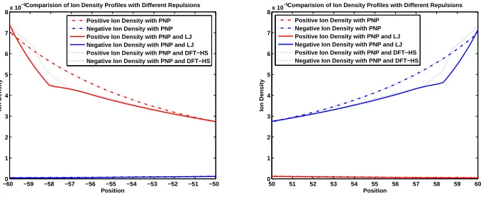
Fig. 4.2.The zoom-in pictures of the left-hand side picture in Figure 4.1 near boundary.

electrostatic potential are chosen such as

φ−η∂φ ∂x

x=−60

=

φ+η∂φ ∂x

x=60

= 0.

This simple situation shows a finite size effect. We compare modified and pure PNP equations with the same computational condition except the repulsion term. The comparison of these results is presented in the right-hand side panel of Figure 4.1. The left-hand side panel in Figure 4.1 is for the ion density profiles of PNP system without any finite size effects for clarification. According to the results, both numerical solutions to PNP with LJ repulsive potential and with DFT hard sphere potential have the same overall behavior of ion concentration, but in detail the ion concentrations show a different profile, especially, the difference near the boundary is larger than that in bulk. In this case, the largest contribution of the repulsion term is apparent near the boundary. It is caused by the high concentration of ions near boundary obeying the electrostatic field. For more detail behavior of the solutions, the zoom-in panels in Figure 4.2 show the behavior of the solutions in more detail. One can easily observe that the DFT hard sphere potential gives a more complex behavior than the

[image:11.612.86.425.298.440.2]

(12)

LJ repulsive potential.

Next, we consider a little more complicated situation which has a charged wall. The right-hand side boundary/wall is negatively charged. The left-hand side bound-ary/wall has no charge. We establish the charged wall through the variable, ρ0 in Poisson equation (2.2). We set ρ0 = 0 on the left-hand side boundary, and ρ0 = 1 on the other side boundary. The domain Ω is [−10,10]. In this case, we impose the Dirichlet and Neumann boundary conditions for the left-hand side and the right-hand side boundary, respectively.

φ|_x₌₋₁₀= 0, ∂φ ∂~ν

x=10

= 0

where~ν is the unit outer normal vector.

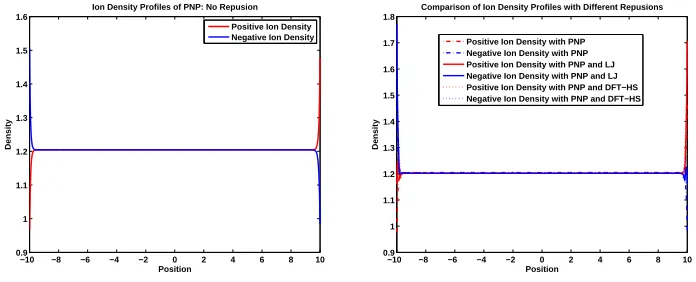
The numerical results with one-side charged wall is presented in Figure 4.3. The left-hand side panel in Figure 4.3 is the ion concentration profiles without any finite size effects and the right-hand side panel is those with the finite size effects. The results on the right-hand side panel shows very important phenomena of the finite size effects, so called, the layering phenomena (charge inversion). The comparison shows a rigorous evidence of the finite size effects in the modified PNP system.

−10 −8 −6 −4 −2 0 2 4 6 8 10

0.9 1 1.1 1.2 1.3 1.4 1.5 1.6

Ion Density Profiles of PNP: No Repusion

Position

Density

Positive Ion Density Negative Ion Density

−10 −8 −6 −4 −2 0 2 4 6 8 10

0.9 1 1.1 1.2 1.3 1.4 1.5 1.6 1.7 1.8

Comparison of Ion Density Profiles with Different Repusions

Position

Density

[image:12.612.78.426.334.475.2]

Fig. 4.3. The ionic concentration profile without finite size effects (left), and the

com-parison of ionic concentrations with the finite size effects, LJ repulsive potential and DFT hard sphere potential (right) under the no-flux boundary condition.

For more detailed comparison, we present the zoom-in pictures near the bound-aries in Figure 4.4. One can easily see the contribution of the finite size effects and the difference between the PNP and the modified PNP equations. The DFT hard sphere potential gives more complex behavior than the LJ repulsive potential.

5. Conclusion. We have introduced a mathematical model system, modified PNP, for ionic solutions including hard sphere repulsion. The modified PNP has been derived from the energy dissipation law using the energetic variational approach. We also present some numerical results showing the finite size effects in modified PNP equations.

(13)

−10 −9.95 −9.9 −9.85 −9.8 −9.75 −9.7 −9.65 −9.6 0.9

1 1.1 1.2 1.3 1.4 1.5 1.6 1.7 1.8

Position

Density

9.6 9.65 9.7 9.75 9.8 9.85 9.9 9.95

0.9 1 1.1 1.2 1.3 1.4 1.5 1.6 1.7 1.8

Position

Density

[image:13.612.83.425.99.239.2]

Fig. 4.4. The zoom-in pictures of the left-hand side picture in Figure 4.3 near boundary

The model and calculations might be improved by using another type of repulsive potential instead of the Lennard-Jones or DFT hard sphere repulsion potentials we use here. Moreover, the comparison of PNP equations with different types of repulsive potentials would also reveal interesting physics and biophysics.

Acknowledgement. We would like to thank Professor Dezs˝o Boda, Dirk Gille-spie, and Roland Roth for a communication on the DFT related to the hard sphere repulsion. Chun Liu is supported by NSF grant DMS-0707594. Bob Eisenberg was supported in part by NIH grant GM076013.

Appendix A. The Variational Derivative of The Total Repulsive En-ergy. We here present the detail derivation of the finite size effect terms in (3.17)– (3.18).

δErepulsion = 1

2

Z Z

εn,n(an+an)12

|~x−~y|12 δcn(~x)cn(~y)d~xd~y

(A.1) +1

2

Z Z

εn,n(an+an)12

|~x−~y|12 cn(x~)δcn(~y)d~xd~y+ 1 2

Z Z

εn,p(an+ap)12

|~x−~y|12 δcn(~x)cp(~y)d~xd~y.

Therefore, we have the repulsive term,µr

cn, in the chemical potential for

Nernst-Planck equation of the charge densitycn.

µr_c_n=

Z ₁₂

εn,n(an+an)12

|~x−~y|12 cn(~y) +

Z ₆

εn,p(an+ap)12

|~x−~y|12 cp(~y)d~y. (A.2)

Similarly, we have the repulsive term forcp.

µr_c_p =

Z ₁₂_ε

p,p(ap+ap)12

|~x−~y|12 cp(~y) +

Z ₆_ε

p,n(ap+an)12

|~x−~y|12 cn(~y)d~y. (A.3)

REFERENCES

[1] J. D. Jackson,Classical Electrodynamics, 3rd, Wiley, New York, 1998.

[2] C. Lee, H. Lee, Y. Hyon, C. Liu, and T. C. Lin,Renormalized Poisson-Boltzmann Equations:

(14)

[3] P. G. Cialet,The Finite Element Method for Elliptic Equations, North-Holland, Amsterdam, 1978.

[4] F. Brezzi, and M. Fortin,Mixed and hybrid finite element methods, Springer-Verlag, New

York, 1991.

[5] J. Zhang, X. Gong, C. Liu, W. Wen, and P. Sheng,Electrorheological Fluid Dynamics,

PRL, 101, pp.194503-1–4, 2008.

[6] R. Ryham,An Energetic Variational Approach To Mathematical Modeling Of Charged Fluids:

Charge Phases, Simulation And Well Posedness, thesis, Pennsylvania State University, 2006.

[7] J. Xu, and L. Zikatanov, A Monotone Finite Element Scheme For Convection-Diffusion

Equations, Math. Comp., 68(228), pp.1429–1446, 1999.

[8] F. Brezzi, L. D. Marini, S. Micheletti, P. Pietra, R. Sacco, and S. Wang,Finite element

and finite volume discretizations of Drift-Diffusion type fluid models for semiconductors, Centre National de la Recherche Scientifique Paris, France, Technical Report, pp.2002– 1302, 2002.

[9] R. Ryham, C. Liu, and L. Zikatanov,An Mathematical Models for the Deformation of

Elec-trolyte Droplets, Discrete Contin. Dyn. Syst. Ser. B 8, no. 3, p. 649–661, 2007.

[10] R. Ryham, C. Liu and Z. Q. Wang,On electro-kinetic fluids: one dimensional configurations,

Discrete Contin. Dyn. Syst. Ser. B 6, no. 2, p. 357–371, 2006.

[11] J. Zhang, X. Gong, C. Liu, W. Wen, and P. Sheng,Electrorheological Fluid Dynamics,

Phys. Review Lett., 101(19), pp.194503-1–4, 2008.

[12] Y. Hyon, D. Y. Kwak and C. Liu,Energetic Variational Approach in Complex Fluids:

Max-imum Dissipation Principle, DCDS-A, Vol.24, No.4, pp.1291–1304, 2010.

[13] P. A. Markowich,The Stationary Seminconductor Device Equations, Springer-Verlag,

Vi-enna, 1986.

[14] J. H. Park and J. W. Jerome,Qualitative properties of steady-state Poisson-Nernst-Planck

systems: mathematical study, SIAM J. APPL. MATH. Vol.57, No.3, pp.609–630, 1997.

[15] B. Eisenberg,Ionic Channels in Biological Membranes: Natural Nanotubes, Acc. Chem. Res.,

31, pp.117–123, 1998.

[16] W. Nonner, D. P. Chen, and B. Eisenberg,Progress and Prospects in Permeation, J. Gen.

Physiol., 113, pp.773–782, 1999.

[17] D. Boda, W. Nonner, M. Valisk´o , D. Henderson, B. Eisenberg, and D. Gillespie,Steric

Selectivity in Na Channels Arising from Protein Polarization and Mobile Side Chains, Biophys. J., 93, pp.1960–1980, 2007.

[18] B. Eisenberg, Y. Hyon, and C. Liu,Energy Variational Analysis EnVarA of Ions in Water

and Channels: Field Theory for Primitive Models of Complex Ionic Fluids, preprint, 2010.

[19] P. Graf, M. G. Kurikova, R. D. Coalson, and A. Nitzan,Comparison of Dynamic Lattice

Monte Carlo Simulations and the Dielectric Selt-Energy Poisson-Nernst-Planck Contin-uum Theory for Model Ion Channels, J. Phys. Chem. B, 108, pp.2006–2015, 2004.

[20] R. D. Coalson, and M. G. Kurikova,Poisson-Nernst-Planck Theory Approach to the

Calcu-lation of Current Through Biological Ion Channels, IEEE Transaction on NanoBioscience, 4, pp.81–93, 2005.

[21] M. S. Kilic. and M. Z. Bazant,Steric effects in the dynamics of electrolytes at large applied

voltages. II. Modified Poisson-Nernst-Planck equations, Phys. Review E 75, pp.021503-1– 11, 2007.

[22] A. L. Hodgkin, and A. F. Huxley,A Qualitative Description of the Membrane Current and

Its Application to Conduction and Excitation in Nerve, J. Physiology, 117, pp.500–544, 1952.

[23] J. P. Keener and J. Sneyd,Mathematical Physiology, Springer-Verlag, New York, 1998.

[24] B. Hille,Ion channels of excitable membranes, 3rd Edition, Sinauer Associates, Inc., 2001.

[25] D. Purves,Neuroscience, 4th Edition, Sinauer Associates, Inc., 2007.

[26] C. Koch,Biophysics of computation, Oxford University Press, New York, 2004.

[27] Y. Mori, J .W. Jerome, and C. S. Peskin,A Three-dimensional Model of Cellular Electrical

Activity, Bulletin of the Institute of Mathematics Academia Sinica, 2(2), pp.367–390, 2007.

[28] Y. Mori,A Three-Dimensional Model of Cellular Electrical Activity, PhD thesis, New York

University, 2007.

[29] J. K. Percus,Equilibrium State of a Classical Fluid of Hard Rods in an External Field, J.

Stat. Phys. 15, pp.505–511, 1976.

[30] T. K. Vanderlick, H. T. Davis, and J. K. Percus,The statistical mechanics of

inhomoge-neous hard rod mixtures, J. Chem. Phys. 91(11), pp.7136–7145, 1989.

[31] J. P. Hansen and I. R. McDonald,Theory of Simple Liquids, Academic Press, London, 1986.

(15)

Chem. Phys. 51(2), pp.635–636, 1969.

[33] J. K. Percus and G. J. Yevick, Analysis of Classical Statistical Mechanics by Means of

Collective Coordinates, Phys. Rev. 110(1), pp.1–13, 1958.

[34] J. C. Lebowitz,Exact Solution of Generalized Percus-Yevick Equation for a Mixture of Hard

Spheres, Phys. Rev. 133(4A), pp.A895–899, 1964.

[35] Y. Rosenfeld, Free-Energy Model for the Inhomogeneous Hard-Sphere Fluid Mixture and

Density-Functional Theory of Freezing, Phys. Rev. Lett, 63(9), pp.980–983, 1989.

[36] Y. Rosenfeld,Free-Energy Model for the Inhomogeneous Hard-Sphere Fluid in D dimensions:

Structure factors for the hard-disk (D= 2) mixtures in simple explicit form, Phys. Rev. A, 42(10), pp.5978–5989, 1990.

[37] H. Hansen-Goos, and R. Roth,A New Generalization of the Carnahan-Starling Equation of

State to Additive Mixtures of Hard Spheres, J. Chem. Phys., 124, pp.154506-1–8, 2006.

[38] R. Roth,Fundamental measure theory for hard-sphere mixtures: a review, Journal of Physics:

Condensed Matter, 22(6), pp.063102-1–18, 2010.

[39] D. Gillespie, M. Valisk´o and D. Boda,Density functional theory of the electrical double

layer: the RFD functional, J. Phys.: Condens. Matter, 17, pp.6609–6626, 2005.

[40] D. Gillespie,Energetics of divalent selectivity in a calcium channel: the ryanodine receptor

case study, Biophys. J., 94(4), pp.1169–1184, 2008.

[41] J. Barthel, H. Krienke, and W. Kunz,Physical Chemistry of Electrolyte Solutions: Modern

Aspects, Springer-Verlag, New York, 1998.

[42] W. R. Fawcett,Liquids, Solutions, and Interfaces: From Classical Macroscopic Descriptions

to Modern Microscopic Details, Oxford University Press, New York, 2004.

[43] L. L. Lee,Molecular Thermodynamics of Electrolyte Solutions, World Scientific, Singapore,

2008.

[44] K. S. Pitzer,Thermodynamics, McGraw Hill, New York, 1995.

[45] M. Z. Bazant, K. Thornton, and A. Ajdari,Diffuse-charge dynamics in electrochemical

systems, Physical Review E, 70, pp.021506-1–24, 2004.

[46] IBM Research,Damocles Web Site: http://www.research.ibm.com/DAMOCLES/home.html.,

2007.

[47] B. Eisenberg, Living Transistors: a Physicist’s View of Ion Channels. Version 2.,

http://arxiv.org/abs/q-bio/0506016v2 , pp.1–24, 2008.

[48] R. Eisenberg, and D. Chen,Poisson-Nernst-Planck (PNP) theory of an open ionic channel,

Biophysical J., 64:A22, 1993.

[49] J. W. Jerome,Analysis of Charge Transport. Mathematical Theory and Approximation of

Semiconductor Models, Springer-Verlag, New York, 1995.

[50] P. A. Markowich, C. A. Ringhofer, and C. Schmeiser,Semiconductor Equations,

Springer-Verlag, New York, 1990.

[51] S. Selberherr, Analysis and Simulation of Semiconductor Devices, Springer-Verlag, New

York, 1984.

[52] Y. Rosenfeld,Geometrically based density-functional theory for confined fluids of asymmetric

(“complex”) molecules, Chemical Applications of Density-Functional Theory. B. B. Laird, R. B. Ross and T. Ziegler. Washington, D.C., American Chemical Society, 629, pp.198–212, 1966.

[53] Y. Rosenfeld, and L. Blum,Statistical Mechanics of Charged objects: General method and

application to simple systems, J. Chem. Phys., 85, pp.1556–1566, 1986.

[54] Y. Rosenfeld, and M. Schmidt, H. L. Wen and P. Tarazona,Fundamental-measure

free-energy density functional for hard spheres: Dimensional crossover and freezing, Physical Review E, 55, pp.4245–4263, 1997.

[55] R. Evans,Density Functionals in the Theory of Nonuniform Fluids, Fundamentals of

Inho-mogeneous Fluids. D. Henderson. Marcel Dekker: 606, New York, 1992.

[56] D. Gillespie, W. Nonner and R. S. Eisenberg,Coupling Poisson-Nernst-Planck and

Den-sity Functional Theory to Calculate Ion Flux, Journal of Physics: Condensed Matter, 14, pp.12129–12145, 2002.

[57] D. Henderson,Fundamentals of Inhomogeneous Fluids, Marcel Dekker, New York, 1992.

[58] R. M. Accascina, and R. M. Fuoss,Electrolytic Conductance, Interscience, New York, 1959.

[59] R. M. Fuoss, and L. Onsager,Conductance of Strong Electrolytes at Finite Dilutions, Proc.

Natl. Acad. Sci., 41(5), pp.274–283, 1955.

[60] J. C. Justice,Conductance of Electrolyte Solutions, Comprehensive Treatise of

Electrochem-istry Volume 5 Thermondynbamic and Transport Properties of Aqueous and Molten Elec-trolytes. B. E. Conway, J. O. M. Bockris and E. Yaeger. Plenum, New York, pp.223-338, 1983.