Generative Bridging Network for Neural Sequence Prediction

Proceedings of NAACL-HLT 2018, pages 1706–1715

Generative Bridging Network for Neural Sequence Prediction

Wenhu Chen,1 _{Guanlin Li,}2_{Shuo Ren,}5 _{Shujie Liu,}3 _{Zhirui Zhang,}4_{Mu Li,}3 _{Ming Zhou}3 University of California, Santa Barbara1

Harbin Institute of Technology2 Microsoft Research Asia3

University of Science and Technology of China4 Beijing University of Aeronautics and Astronautics5

[email protected] [email protected]{v-shure, shujliu, v-zhirzh, muli, mingzhou}@microsoft.com

Abstract

In order to alleviate data sparsity and over-fitting problems in maximum likelihood esti-mation (MLE) for sequence prediction tasks, we propose the Generative Bridging Network (GBN), in which a novel bridge module is in-troduced to assist the training of the sequence prediction model (the generator network). Un-like MLE directly maximizing the conditional likelihood, the bridge extends the point-wise ground truth to a bridge distribution condi-tioned on it, and the generator is optimized to minimize their KL-divergence. Three different GBNs, namely uniform GBN, language-model GBN and coaching GBN, are proposed to pe-nalize confidence, enhance language smooth-ness and relieve learning burden. Experiments conducted on two recognized sequence predic-tion tasks (machine translapredic-tion and abstractive text summarization) show that our proposed GBNs can yield significant improvements over strong baselines. Furthermore, by analyz-ing samples drawn from different bridges, ex-pected influences on the generator are verified. 1 Introduction

Sequence prediction has been widely used in tasks where the outputs are sequentially structured and mutually dependent. Recently, massive explo-rations in this area have been made to solve prac-tical problems, such as machine translation (Bah-danau et al.,2014;Ma et al.,2017;Norouzi et al., 2016), syntactic parsing (Vinyals et al., 2015), spelling correction (Bahdanau et al.,2014), image captioning (Xu et al., 2015) and speech recogni-tion (Chorowski et al., 2015). Armed with mod-ern computation power, deep LSTM (Hochreiter and Schmidhuber, 1997) or GRU (Chung et al., 2014) based neural sequence prediction models have achieved the state-of-the-art performance.

The typical training algorithm for sequence prediction is Maximum Likelihood Estimation

𝑥1 𝑥2

𝐴𝑡𝑡

𝑥𝑇

𝑦1𝑗 𝑦2𝑗 𝑦𝑇𝑗𝑗

𝑠 𝑦₁𝑗 𝑦_𝑇𝑗𝑗₋₁

𝑿

𝒀𝒋

𝑦1∗ 𝑦2∗ 𝑦𝑇∗′ 𝒀∗

𝒀𝒋

𝑃𝜂(𝑌|𝑌∗)

𝑦1𝑗 𝑦2𝑗 𝑦𝑇𝑗𝑗

𝐵𝑟𝑖𝑑𝑔𝑒 𝑚𝑜𝑑𝑢𝑙𝑒

𝐺𝑒𝑛𝑒𝑟𝑎𝑡𝑜𝑟 𝑛𝑒𝑡𝑤𝑜𝑟𝑘

𝒀𝟏_{… …𝒀}𝑲

𝑃𝜃(𝑌|𝑋)

𝐵𝑟𝑖𝑑𝑔𝑒 𝑠𝑎𝑚𝑝𝑙𝑒𝑠

…

…

…

…

…

…

…

Figure 1: The overall architecture of our novel Gen-erative Bridging Network (GBN). Two main compo-nents, namely the generator network and the bridge module, are connected through samples (Y1_{. . . Y}K _in

red) from the bridge module during training time. (We sometimes call them generator and bridge in brief re-spectively in the following discussion.) The generator is implemented through an attentive encoder-decoder, where in the figureAttrepresents the attention module.

(MLE), which maximizes the likelihood of the tar-get sequences conditioned on the source ones:

✓⇤= argmax

✓ (X,YE⇤)⇠D

logp✓(Y⇤|X) (1)

Despite the popularity of MLE or teacher forc-ing (Doya, 1992) in neural sequence prediction tasks, two general issues are always haunting: 1). data sparsity and 2). tendency for overfitting, with which can both harm model generalization.

To combat data sparsity, different strategies have been proposed. Most of them try to take advantage of monolingual data (Sennrich et al., 2015;Zhang and Zong,2016;Cheng et al.,2016). Others try to modify the ground truth target based on derived rules to get more similar examples for training (Norouzi et al., 2016; Ma et al., 2017). To alleviate overfitting, regularization techniques,

such as confidence penalization (Pereyra et al., 2017) and posterior regularization (Zhang et al., 2017), are proposed recently.

As shown in Figure1, we propose a novel learn-ing architecture, titled Generative Bridglearn-ing Net-work (GBN), to combine both of the benefits from synthetic data and regularization. Within the ar-chitecture, the bridge module (bridge) first trans-forms the point-wise ground truth into a bridge distribution, which can be viewed as a target pro-poser from whom more target examples are drawn to train the generator. By introducing different constraints, the bridge can be set or trained to pos-sess specific property, with which the drawn sam-ples can augment target-side data (alleviate data sparsity) while regularizing the training (avoid overfitting) of the generator network (generator).

In this paper, we introduce three different con-straints to build three bridge modules. Together with the generator network, three GBN systems are constructed: 1). a uniform GBN, instantiating the constraint as a uniform distribution to penal-ize confidence; 2). a language-model GBN, in-stantiating the constraint as a pre-trained neural language model to increase language smoothness; 3). a coaching GBN, instantiating the constraint as the generator’s output distribution to seek a close-to-generator distribution, which enables the bridge to draw easy-to-learn samples for the generator to learn. Without any constraint, our GBN degrades to MLE. The uniform GBN is proved to minimize KL-divergence with a so-called payoff distribution as in reward augmented maximum likelihood or RAML (Norouzi et al.,2016).

Experiments are conducted on two sequence prediction tasks, namely machine translation and abstractive text summarization. On both of them, our proposed GBNs can significantly improve task performance, compared with strong base-lines. Among them, the coaching GBN achieves the best. Samples from these three different bridges are demonstrated to confirm the expected impacts they have on the training of the generator. In summary, our contributions are:

• A novel GBN architecture is proposed for se-quence prediction to alleviate the data spar-sity and overfitting problems, where the bridge module and the generator network are integrated and jointly trained.

• Different constraints are introduced to build GBN variants: uniform GBN,

language-model GBN and coaching GBN. Our GBN architecture is proved to be a generalized form of both MLE and RAML.

• All proposed GBN variants outperform the MLE baselines on machine translation and abstractive text summarization. Similar rela-tive improvements are achieved compared to recent state-of-the-art methods in the trans-lation task. We also demonstrate the advan-tage of our GBNs qualitatively by comparing ground truth and samples from bridges.

𝐶𝑜𝑛𝑠𝑡𝑟𝑎𝑖𝑛𝑡

𝐺𝑒𝑛𝑒𝑟𝑎𝑡𝑜𝑟 𝐵𝑟𝑖𝑑𝑔𝑒

Regularization-by-synthetic-samples 𝑌∗

𝑝𝐶(𝑌) 𝑆(𝑌, 𝑌∗₎

𝐶(𝑝𝜂, 𝑝𝑐)

Knowledge injection

𝑃𝜂(𝑌|𝑌∗)

𝐾𝐿(𝑝𝜂, 𝑝𝜃) _𝑝 𝜃(𝑌|𝑋)

𝑌∗ 𝑝𝐶(𝑌)

Figure 2: Conceptual interpretation of our Generative Bridging Network (GBN). See detailed discussion in the beginning of Sec.2.

2 Generative Bridging Network

In this section, we first give a conceptual interpre-tation of our novel learning architecture which is sketched in Figure2. Since data augmentation and regularization are two golden solutions for tack-ling data sparsity and overfitting issues. We are willing to design an architecture which can inte-grate both of their benefits. The basic idea is to use a so-called bridge which transformsY⇤to an

easy-to-sample distribution, and then use this distribu-tion (samples) to train and meanwhile regularize the sequence prediction model (the generator).

The bridge is viewed as a conditional distribu-tion1 _p

⌘(Y|Y⇤) to get more target Ys given Y⇤

so as to construct more training pairs(X, Y). In

the meantime, we could inject (empirical) prior knowledge into the bridge through its optimiza-tion objective which is inspired by the design of the payoff distribution in RAML. We formulate the optimization objective with two parts in Equa-tion (2): a) an expected similarity score com-puted through a similarity score functionS(_·, Y⇤)

interpolated with b) a knowledge injection con-straint2_C(p

⌘(Y|Y⇤), pc(Y))where↵controls the

1_{⌘should be treated as an index of the bridge distribution,}

so it is not necessarily the parameters to be learned.

2_{Note that, in our paper, we specifyCto be KL-divergence}

dis-strength of the regularization, formally, we write the objective functionLB(⌘)as follows:

LB(⌘) =

E

Y⇠p⌘(Y|Y⇤)

[ S(Y, Y⇤)] +↵C(p⌘(Y|Y⇤), pc(Y))

(2)

Minimizing it empowers the bridge distribution not only to concentrate its mass around the ground truth Y⇤ but also to adopt certain hope property frompc(Y). With the constructed bridge

distribu-tion, we optimize the generator networkP✓(Y|X)

to match its output distribution towards the bridge distribution by minimizing their KL-divergence:

LG(✓) =KL(p⌘(Y|Y⇤)||p✓(Y|X)) (3)

In practice, the KL-divergence is approximated through sampling process detailed in Sec. 2.3. As a matter of fact, the bridge is the crux of the integration: it synthesizes new targets to allevi-ate data sparsity and then uses the synthetic data as regularization to overcome overfitting. Thus a regularization-by-synthetic-example approach, which is very similar to the prior-incorporation-by-virtual-example method (Niyogi et al.,1998).

2.1 Generator Network

Our generator network is parameterized with the commonly used encoder-decoder architec-ture (Bahdanau et al.,2014;Cho et al.,2014). The encoder is used to encode the input sequence X

to a sequence of hidden states, based on which an attention mechanism is leveraged to compute context vectors at the decoding stage. The con-text vector together with previous decoder’s hid-den state and previously predicted label are used, at each time step, to compute the next hidden state and predict an output label.

As claimed in Equation (3), the generator net-work is not trained to maximize the likelihood of the ground truth but tries best to match the bridge distribution, which is a delegate of the ground truth. We use gradient descent to optimize the KL-divergence with respect to the generator:

rLG(✓) = E

Y⇠p⌘(Y|Y⇤)

logrp✓(Y|X) (4)

The optimization process can be viewed as the generator maximizing the likelihood of samples

tributionpc, however, we believe mathematical form ofCis

not restricted, which could motivate further development.

drawn from the bridge. This may alleviate data sparsity and overfitting by posing more unseen scenarios to the generator and may help the gen-erator generalize better in test time.

2.2 Bridge Module3

Our bridge module is designed to transform a single target example Y⇤ to a bridge

distribu-tion p⌘(Y|Y⇤). We design its optimization

tar-get in Equation (2) to consist of two terms, namely, a concentration requirement and a con-straint. The constraint is instantiated as KL-divergence between the bridge and a contraint dis-tributionpc(Y). We transform Equation (2) as

fol-lows, which is convenient for mathematical ma-nipulation later:

LB(⌘) =

E

Y⇠p⌘

[ S(Y, Y⇤)

⌧ ] +KL(p⌘(Y|Y ⇤_)||p

c(Y))

(5)

S(Y, Y⇤) is a predefined score function which

measures similarity betweenY andY⇤ and peaks

when Y = Y⇤, while pc(Y)reshapes the bridge

distribution. More specifically, the first term en-sures that the bridge should concentrate around the ground truthY⇤, and the second introduces willing

property which can help regularize the generator. The hyperparameter⌧can be interpreted as a

tem-perature which scales the score function. In the following bridge specifications, the score function

S(Y, Y⇤)is instantiated according to Sec.3.1.

1. Delta Bridge The delta bridge can be seen as the simplest case where ↵ = 0 or no

con-straint is imposed. The bridge seeks to minimize

E

Y⇠p⌘(Y|Y⇤)

[ S(Y,Y_⌧ ⇤)]. The optimal solution is when the bridge only samplesY⇤, thus the Dirac

delta distribution is described as follows:

p⌘(Y|Y⇤) = Y⇤(Y) (6)

This exactly corresponds to MLE, where only ex-amples in the dataset are used to train the genera-tor. We regard this case as our baseline.

2. Uniform Bridge The uniform bridge adopts a uniform distribution U(Y) as constraint. This

3_{Although we name it bridge module, we explicitly learn}

bridge motivates to include noise into target exam-ple, which is similar to label smoothing (Szegedy et al.,2016). The loss function can be written as:

LB(⌘) =

E

Y⇠p⌘

[ S(Y, Y ⇤₎

⌧ ] +KL(p⌘(Y|Y

⇤_)||U(Y))

(7)

We can re-write it as follows by adding a constant to not change the optimization result:

LB(⌘) +C =KL(p⌘(Y|Y⇤)||

expS(Y,Y_⌧ ⇤)

Z )

(8)

This bridge is static for having a closed-form so-lution:

p⌘(Y|Y⇤) =

expS(Y,Y_⌧ ⇤)

Z (9)

where Z is the partition function. Note that our

uniform bridge corresponds to the payoff distribu-tion described in RAML (Norouzi et al.,2016).

3. Language-model (LM) Bridge The LM

bridge utilizes a pretrained neural language model

pLM(Y)as constraint, which motivates to propose

target examples conforming to language fluency.

LB(⌘) =

E

Y⇠p⌘(Y|Y⇤)

[ S(Y, Y⇤)

⌧ ] +KL(p⌘(Y|Y ⇤_)||p

LM)

(10)

Similar to the uniform bridge case, we can re-write the loss function to a KL-divergence:

LB(⌘) +C

=KL(p⌘(Y|Y⇤)||

pLM(Y)·expS(Y,Y

⇤₎

⌧

Z )

(11)

Thus, the LM bridge is also static and can be seen as an extension of the uniform bridge, where the exponentiated similarity score is re-weighted by a pretrained LM score, and renormalized:

p(Y_|Y⇤) = pLM(Y) exp

S(Y,Y⇤₎

⌧

Z (12)

whereZis the partition function. The above

equa-tion looks just like the payoff distribuequa-tion, whereas an additional factor is considered.

4. Coaching Bridge The coaching bridge uti-lizes the generator’s output distribution as con-straint, which motivates to generate training sam-ples which are easy to be understood by the generator, so as to relieve its learning burden. The coaching bridge follows the same spirit as the coach proposed in Imitation-via-Coaching (He et al.,2012), which, in reinforcement learning vo-cabulary, advocates to guide the policy (genera-tor) with easy-to-learn action trajectories and let it gradually approach the oracle when the optimal action is hard to achieve.

LB(⌘) =

E

Y⇠p⌘

[ S(Y, Y⇤)

⌧ ] +KL(p✓(Y|X)||p⌘(Y|Y ⇤₎₎

(13)

Since the KL constraint is a moving target when the generator is updated, the coaching bridge should not remain static. Therefore, we perform iterative optimization to train the bridge and the generator jointly. Formally, the derivatives for the coaching bridge are written as follows:

rLB(⌘) = E Y⇠p⌘

[ S(Y, Y⇤)

⌧ rlogp⌘(Y|Y ⇤_)]

+ E

Y⇠p✓r

logp⌘(Y|Y⇤)

(14)

The first term corresponds to the policy gradient algorithm described in REINFORCE (Williams, 1992), where the coefficient S(Y, Y⇤)/⌧

corre-sponds to reward function. Due to the mutual de-pendence between bridge module and generator network, we design an iterative training strategy, i.e. the two networks take turns to update their own parameters treating the other as fixed.

2.3 Training

The training of the above three variants is illus-trated in Figure3. Since the proposed bridges can be divided into static ones, which only require pre-training, and dynamic ones, which require contin-ual training with the generator, we describe their training process in details respectively.

2.3.1 Stratified-Sampled Training

Generator 𝑝_𝜃(𝑌|𝑋) 𝑝_{𝑑𝑎𝑡𝑎}(𝑌∗₎

LM Bridge

𝑝_𝜂(𝑌|𝑌∗₎ Coach Bridge_𝑝

𝜂(𝑌|𝑌∗) 𝑈(𝑌)

Iterative Training Stratified-sampled

Training

Uniform Bridge

𝑝_𝜂(𝑌|𝑌∗₎ 𝑝_𝐿𝑀(𝑌)

Pre-trained

Figure 3: The training processes of the three different variants of our GBN architecture (Sec.2.3).

due to the intractability of these bridge distribu-tions, direct sampling is infeasible. Therefore, we followNorouzi et al.(2016);Ma et al.(2017) and adopt stratified sampling to approximate the direct sampling process. Given a sentenceY⇤, we first

sample an edit distancem, and then randomly

se-lectmpositions to replace the original tokens. The

difference between the uniform and the LM bridge lies in that the uniform bridge replaces labels by drawing substitutions from a uniform distribution, while LM bridge takes the history as condition and draws substitutions from its step-wise distribution.

2.3.2 Iterative Training

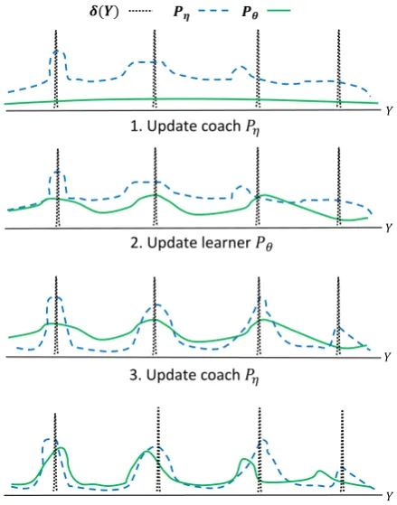
Since the KL-constraint is a moving target for the coaching bridge, an iterative training strategy is designed to alternately update both the generator and the bridge (Algorithm 1). We first pre-train both the generator and the bridge and then start to alternately update their parameters. Figure4 intu-itively demonstrates the intertwined optimization effects over the coaching bridge and the generator. We hypothesize that iterative training with easy-to-learn guidance could benefit gradient update, thus result in better local minimum.

3 Experiment

We select machine translation and abstractive text summarization as benchmarks to verify our GBN framework.

3.1 Similarity Score Function

In our experiments, instead of directly using BLEU or ROUGE as reward to guide the bridge network’s policy search, we design a simple

sur-𝑷𝜼 𝑷𝜽

𝑌

2. Update learner 𝑃𝜃

𝑌

4. Update learner 𝑃𝜃

1. Update coach 𝑃𝜂

𝑌

3. Update coach 𝑃𝜂

𝑌

𝜹(𝒀)

Figure 4: Four iterative updates of the coaching bridge and the generator. In an early stage, the pre-trained generatorP✓may not put mass on some ground truth

target points within the output space, shown by (Y).

The coaching bridge is first updated with Equation (14) to locate in between the Dirac delta distribution and the generator’s output distribution. Then, by sampling from the coaching bridge for approximating Equation (4), target samples which demonstrate easy-to-learn se-quence segments facilitate the generator to be opti-mized to achieve closeness with the coaching bridge. Then this process repeats until the generator converges.

rogate n-gram matching reward as follows:

S(Y, Y⇤) = 0.4_⇤N4+0.3⇤N3+0.2⇤N2+0.1⇤N1 (15)

Nnrepresents the n-gram matching score between Y andY⇤. In order to alleviate reward sparsity at

sequence level, we further decompose the global rewardS(Y, Y⇤)as a series of local rewards at

ev-ery time step. Formally, we write the step-wise rewards(yt|y1:t 1, Y⇤)as follows:

s(yt|y1:t 1, Y⇤) =

8 > > > > > < > > > > > :

1.0;N(y1:t, yt 3:t)N(Y⇤, yt 3:t) 0.6;N(y1:t, yt 2:t)N(Y⇤, yt 2:t) 0.3;N(y1:t, yt 1:t)N(Y⇤, yt 1:t) 0.1;N(y1:t, yt)N(Y⇤, yt)

0.0;otherwise

(16)

whereN(Y,Y˜)represents the occurrence of

Algorithm 1Training Coaching GBN

procedurePRE-TRAINING

Initializep✓(Y|X)andp⌘(Y|Y⇤)with

ran-dom weights✓and⌘

Pre-trainp✓(Y|X)to predictY⇤ given X

Use pre-trained p✓(Y|X) to generate Yˆ

given X

Pre-trainp⌘(Y|Y⇤)to predictYˆ givenY⇤ end procedure

procedureITERATIVE-TRAINING

whileNot Convergeddo

Receive a random example(X, Y⇤) ifBridge-stepthen

Draw samplesY fromp✓(Y|X)

Update bridge via Equation (14)

else ifGenerator-stepthen

Draw samplesY fromp⌘(Y|Y⇤)

Update generator via Equation (4)

end if end while end procedure

a certain sub-sequence yt n+1:t from Y appears

less times than in the referenceY⇤,ytreceives

re-ward. Formally, we rewrite the step-level gradient for each sampledY as follows:

S(Y, Y⇤)

⌧ rlogp⌘(Y|Y ⇤₎

=X

t

s(yt|y1:t 1, Y⇤)

⌧ · rlogp⌘(yt|y1:t 1, Y ⇤₎

(17)

3.2 Machine Translation

Dataset We follow Ranzato et al. (2015); Bah-danau et al.(2016) and select German-English ma-chine translation track of the IWSLT 2014 eval-uation campaign. The corpus contains sentence-wise aligned subtitles of TED and TEDx talks. We use Moses toolkit (Koehn et al.,2007) and remove sentences longer than 50 words as well as lower-casing. The evaluation metric is BLEU (Papineni et al.,2002) computed via the multi-bleu.perl.

System Setting We use a unified GRU-based RNN (Chung et al.,2014) for both the generator and the coaching bridge. In order to compare with existing papers, we use a similar system setting with 512 RNN hidden units and 256 as embed-ding size. We use attentive encoder-decoder to build our system (Bahdanau et al., 2014). Dur-ing trainDur-ing, we apply ADADELTA (Zeiler,2012)

Methods Baseline Model

MIXER 20.10 21.81 +1.71

BSO 24.03 26.36 +2.33

AC 27.56 28.53 +0.97

Softmax-Q 27.66 28.77 +1.11

Uniform GBN (⌧ = 0.8)

29.10

29.80+0.70

LM GBN

(⌧ = 0.8) 29.90+0.80

Coaching GBN

(⌧ = 0.8) 29.98+0.88

Coaching GBN

(⌧ = 1.2) 30.15+1.05

Coaching GBN

(⌧ = 1.0) 30.18+1.08

Table 1: Comparison with existing works on IWSLT-2014 German-English Machine Translation Task.

70 75 80 85 90 95 100

0 1 2 3 4 5 6 7 8 9 10 11 12 13 14

B

LEU

Epoch (Bridge)

Coaching GBN Learning Curve

31.5 31.6 31.7 31.8 31.9 32 32.1 32.2

0 1 2 3 4 5 6 7 8 9 10 11 12 13 14

B

LEU

Epoch (Generator)

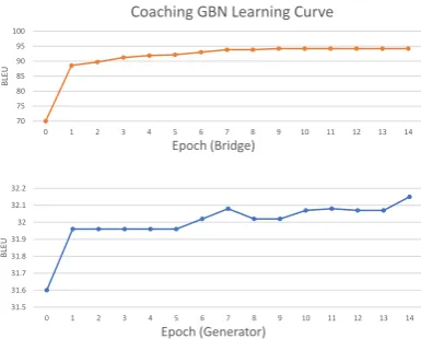
Figure 5: Coaching GBN’s learning curve on IWSLT German-English Dev set.

with ✏ = 10 6 and ⇢ = 0.95 to optimize

pa-rameters of the generator and the coaching bridge. During decoding, a beam size of 8 is used to ap-proximate the full search space. An important hyper-parameter for our experiments is the tem-perature ⌧. For the uniform/LM bridge, we fol-lowNorouzi et al.(2016) to adopt an optimal tem-perature⌧ = 0.8. And for the coaching bridge,

we test hyper-parameters from⌧ _{2 {}0.8,1.0,1.2_}. Besides comparing with our fine-tuned baseline, other systems for comparison of relative BLEU improvement are: MIXER (Ranzato et al.,2015), BSO (Wiseman and Rush,2016), AC (Bahdanau et al.,2016), Softmax-Q (Ma et al.,2017).

over-Methods RG-1 RG-2 RG-L

ABS 29.55 11.32 26.42

ABS+ 29.76 11.88 26.96

Luong-NMT 33.10 14.45 30.71 SAEASS 36.15 17.54 33.63

seq2seq+att 34.04 15.95 31.68 Uniform GBN

(⌧ = 0.8) 34.10 16.70 31.75

LM GBN

(⌧ = 0.8) 34.32 16.88 31.89

Coaching GBN

(⌧ = 0.8) 34.49 16.70 31.95

Coaching GBN

(⌧ = 1.2) 34.83 16.83 32.25

Coaching GBN

(⌧ = 1.0) 35.26 17.22 32.67

Table 2: Full length ROUGE F1 evaluation results on the English Gigaword test set used by (Rush et al.,

2015). RG in the Table denotes ROUGE. Results for comparison are taken from SAEASS (Zhou et al.,

2017).

competing other systems and our proposed GBN can yield a further improvement. We also ob-serve that LM GBN and coaching GBN have both achieved better performance than Uniform GBN, which confirms that better regularization effects are achieved, and the generators become more ro-bust and generalize better. We draw the learning curve of both the bridge and the generator in Fig-ure 5 to demonstrate how they cooperate during training. We can easily observe the interaction between them: as the generator makes progress, the coaching bridge also improves itself to propose harsher targets for the generator to learn.

3.3 Abstractive Text Summarization

Dataset We follow the previous works byRush et al. (2015); Zhou et al. (2017) and use the same corpus from Annotated English Gigaword dataset (Napoles et al.,2012). In order to be com-parable, we use the same script4_{released byRush}

et al. (2015) to pre-process and extract the train-ing and validation sets. For the test set, we use the English Gigaword, released byRush et al.(2015), and evaluate our system through ROUGE (Lin, 2004). Following previous works, we employ ROUGE-1, ROUGE-2, and ROUGE-L as the eval-uation metrics in the reported experimental results.

4_{https://github.com/facebookarchive/NAMAS}

81 81.5 82 82.5 83 83.5

0 1 2 3 4 5 6 7 8 9 10 11 12 13 14

R

O

UGE

-2

Epoch (Bridge)

Coaching GBN Learning Curve

21.7 21.9 22.1 22.3 22.5 22.7

0 1 2 3 4 5 6 7 8 9 10 11 12 13 14

R

O

UGE

-2

Epoch (Generator)

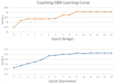
Figure 6: Coaching GBN’s learning curve on Abstrac-tive Text Summarization Dev set.

System Setting We follow Zhou et al. (2017); Rush et al. (2015) to set input and output vo-cabularies to 119,504 and 68,883 respectively, and we also set the word embedding size to 300 and all GRU hidden state size to 512. Then we adopt dropout (Srivastava et al., 2014) with probability p = 0.5 strategy in our out-put layer. We use attention-based sequence-to-sequence model (Bahdanau et al.,2014;Cho et al., 2014) as our baseline and reproduce the results of the baseline reported in Zhou et al. (2017). As stated, the attentive encoder-decode architecture can already outperform existing ABS/ABS+ sys-tems (Rush et al.,2015). In coaching GBN, due to the fact that the input of abstractive summarization

X contains more information than the summary

target Y⇤, directly training the bridge p⌘(Y|Y⇤)

to understand the generatorp✓(Y|X)is infeasible.

Therefore, we design the coaching bridge to re-ceive both source and target input X, Y and we

enlarge its vocabulary size to 88,883 to encom-pass more information about the source side. In Uniform/LM GBN experiments, we also fix the hyper-parameter⌧ = 0.8as the optimal setting.

4 Analysis

By introducing different constraints into the bridge module, the bridge distribution will propose dif-ferent training samples for the generator to learn. From Table3, we can observe that most samples still reserve their original meaning. The uniform bridge simply performs random replacement with-out considering any linguistic constraint. The LM bridge strives to smooth reference sentence with high-frequent words. And the coaching bridge simplifies difficult expressions to relieve genera-tor’s learning burden. From our experimental re-sults, the more rational and aggressive diversifica-tion from the coaching GBN clearly benefits gen-erator the most and helps the gengen-erator generalize to more unseen scenarios.

5 Related Literature

5.1 Data Augmentation and Self-training

In order to resolve the data sparsity problem in Neural Machine Translation (NMT), many works have been conducted to augment the dataset. The most popular strategy is via self-learning, which incorporates the self-generated data directly into training. Zhang and Zong (2016) and Sennrich et al. (2015) both use self-learning to leverage massive monolingual data for NMT training. Our bridge can take advantage of the parallel training data only, instead of external monolingual ones to synthesize new training data.

5.2 Reward Augmented Maximum Likelihood

Reward augmented maximum likelihood or RAML (Norouzi et al., 2016) proposes to in-tegrate task-level reward into MLE training by using an exponentiated payoff distribution. KL divergence between the payoff distribution and the generator’s output distribution are minimized to achieve an optimal task-level reward. Following this work, Ma et al. (2017) introduces softmax Q-Distribution to interpret RAML and reveals its relation with Bayesian decision theory. These two works both alleviate data sparsity problem by augmenting target examples based on the ground truth. Our method draws inspiration from them but seeks to propose the more general Generative Bridging Network, which can transform the ground truth into different bridge distributions, from where samples are drawn will account for different interpretable factors.

System Uniform GBN

Property Random Replacement Reference the questionis, is it worth it ?

Bridge the questionlemon, was it worth it ?

System Language-model GBN

Property Word Replacement Reference nowhow can this help us ?

Bridge sohow can this help us ?

System Coaching GBN

Property Reordering

Reference i needto have a health care lexicon .

Bridge i needa lexicon for health care .

Property Simplification

Reference this is the way thatmost of us were taught

totieour shoes .

Bridge most of us learned tobindour shoes .

Table 3: Qualitative analysis for three different bridge distributions.

5.3 Coaching

Our coaching GBN system is inspired by imita-tion learning by coaching (He et al., 2012). In-stead of directly behavior cloning the oracle, they advocate learning hope actions as targets from a coach which is interpolated between learner’s pol-icy and the environment loss. As the learner makes progress, the targets provided by the coach will become harsher to gradually improve the learner. Similarly, our proposed coaching GBN is moti-vated to construct an easy-to-learn bridge distri-bution which lies in between the ground truth and the generator. Our experimental results confirm its effectiveness to relieve the learning burden.

6 Conclusion

References

Dzmitry Bahdanau, Philemon Brakel, Kelvin Xu, Anirudh Goyal, Ryan Lowe, Joelle Pineau, Aaron Courville, and Yoshua Bengio. 2016. An actor-critic algorithm for sequence prediction. arXiv preprint

arXiv:1607.07086.

Dzmitry Bahdanau, Kyunghyun Cho, and Yoshua Ben-gio. 2014. Neural machine translation by jointly learning to align and translate. arXiv preprint

arXiv:1409.0473.

Yong Cheng, Wei Xu, Zhongjun He, Wei He, Hua Wu, Maosong Sun, and Yang Liu. 2016. Semi-supervised learning for neural machine translation.

arXiv preprint arXiv:1606.04596.

Kyunghyun Cho, Bart Van Merri¨enboer, Caglar Gul-cehre, Dzmitry Bahdanau, Fethi Bougares, Holger Schwenk, and Yoshua Bengio. 2014. Learning phrase representations using rnn encoder-decoder for statistical machine translation. arXiv preprint

arXiv:1406.1078.

Jan K Chorowski, Dzmitry Bahdanau, Dmitriy Serdyuk, Kyunghyun Cho, and Yoshua Bengio. 2015. Attention-based models for speech recogni-tion. InAdvances in Neural Information Processing

Systems. pages 577–585.

Junyoung Chung, Caglar Gulcehre, KyungHyun Cho, and Yoshua Bengio. 2014. Empirical evaluation of gated recurrent neural networks on sequence

model-ing. arXiv preprint arXiv:1412.3555.

Kenji Doya. 1992. Bifurcations in the learning of re-current neural networks. In Circuits and Systems, 1992. ISCAS’92. Proceedings., 1992 IEEE

Interna-tional Symposium on. IEEE, volume 6, pages 2777–

2780.

He He, Jason Eisner, and Hal Daume. 2012. Imitation learning by coaching. InAdvances in Neural

Infor-mation Processing Systems. pages 3149–3157.

Sepp Hochreiter and J¨urgen Schmidhuber. 1997. Long short-term memory. Neural computation

9(8):1735–1780.

Philipp Koehn, Hieu Hoang, Alexandra Birch, Chris Callison-Burch, Marcello Federico, Nicola Bertoldi, Brooke Cowan, Wade Shen, Christine Moran, Richard Zens, et al. 2007. Moses: Open source toolkit for statistical machine translation. In Pro-ceedings of the 45th annual meeting of the ACL on

interactive poster and demonstration sessions.

As-sociation for Computational Linguistics, pages 177– 180.

Chin-Yew Lin. 2004. Rouge: A package for auto-matic evaluation of summaries. InText summariza-tion branches out: Proceedings of the ACL-04 work-shop. Barcelona, Spain, volume 8.

Xuezhe Ma, Pengcheng Yin, Jingzhou Liu, Graham Neubig, and Eduard Hovy. 2017. Softmax q-distribution estimation for structured prediction: A theoretical interpretation for raml. arXiv preprint

arXiv:1705.07136.

Courtney Napoles, Matthew Gormley, and Benjamin Van Durme. 2012. Annotated gigaword. In Pro-ceedings of the Joint Workshop on Automatic Knowl-edge Base Construction and Web-scale KnowlKnowl-edge

Extraction. Association for Computational

Linguis-tics, pages 95–100.

Partha Niyogi, Federico Girosi, and Tomaso Poggio. 1998. Incorporating prior information in machine learning by creating virtual examples. Proceedings

of the IEEE86(11):2196–2209.

Mohammad Norouzi, Samy Bengio, Navdeep Jaitly, Mike Schuster, Yonghui Wu, Dale Schuurmans, et al. 2016. Reward augmented maximum likeli-hood for neural structured prediction. InAdvances

In Neural Information Processing Systems. pages

1723–1731.

Kishore Papineni, Salim Roukos, Todd Ward, and Wei-Jing Zhu. 2002. Bleu: a method for automatic eval-uation of machine translation. In Proceedings of the 40th annual meeting on association for

compu-tational linguistics. Association for Computational

Linguistics, pages 311–318.

Gabriel Pereyra, George Tucker, Jan Chorowski, Łukasz Kaiser, and Geoffrey Hinton. 2017. Regular-izing neural networks by penalRegular-izing confident output distributions. arXiv preprint arXiv:1701.06548. Marc’Aurelio Ranzato, Sumit Chopra, Michael Auli,

and Wojciech Zaremba. 2015. Sequence level train-ing with recurrent neural networks. arXiv preprint

arXiv:1511.06732.

Alexander M Rush, Sumit Chopra, and Jason We-ston. 2015. A neural attention model for ab-stractive sentence summarization. arXiv preprint

arXiv:1509.00685.

Rico Sennrich, Barry Haddow, and Alexandra Birch. 2015. Improving neural machine translation models with monolingual data. arXiv preprint

arXiv:1511.06709.

Nitish Srivastava, Geoffrey E Hinton, Alex Krizhevsky, Ilya Sutskever, and Ruslan Salakhutdinov. 2014. Dropout: a simple way to prevent neural networks from overfitting. Journal of Machine Learning

Re-search15(1):1929–1958.

Christian Szegedy, Vincent Vanhoucke, Sergey Ioffe, Jon Shlens, and Zbigniew Wojna. 2016. Rethinking the inception architecture for computer vision. In

Proceedings of the IEEE Conference on Computer

Oriol Vinyals, Łukasz Kaiser, Terry Koo, Slav Petrov, Ilya Sutskever, and Geoffrey Hinton. 2015. Gram-mar as a foreign language. InAdvances in Neural

Information Processing Systems. pages 2773–2781.

Ronald J Williams. 1992. Simple statistical gradient-following algorithms for connectionist reinforce-ment learning. Machine learning8(3-4):229–256. Sam Wiseman and Alexander M Rush. 2016.

Sequence-to-sequence learning as beam-search op-timization. arXiv preprint arXiv:1606.02960. Kelvin Xu, Jimmy Ba, Ryan Kiros, Kyunghyun Cho,

Aaron Courville, Ruslan Salakhudinov, Rich Zemel, and Yoshua Bengio. 2015. Show, attend and tell: Neural image caption generation with visual at-tention. In International Conference on Machine

Learning. pages 2048–2057.

Matthew D Zeiler. 2012. Adadelta: an adaptive learn-ing rate method.arXiv preprint arXiv:1212.5701. Jiacheng Zhang, Yang Liu, Huanbo Luan, Jingfang Xu,

and Maosong Sun. 2017. Prior knowledge integra-tion for neural machine translaintegra-tion using posterior regularization. In Proceedings of the 55th Annual Meeting of the Association for Computational

Lin-guistics (Volume 1: Long Papers). volume 1, pages

1514–1523.

Jiajun Zhang and Chengqing Zong. 2016. Exploit-ing source-side monolExploit-ingual data in neural machine translation. InEMNLP. pages 1535–1545.