Nonparametric bootstrapping for multiple logistic regression model using R

(1)

NONPARAMETRIC BOOTSTRAPPING FOR MULTIPLE

LOGISTIC REGRESSION MODEL USING R

Ahmed Hossain

Department of Public Health Sciences University of Toronto

Ontario, Canada

and

H. T. Abdullah Khan Department of Statistics

University of Dhaka Dhaka, Bangladesh

ABSTRACT

The use of explanatory variables or covariates in a regression model is an important way to rep-resent heterogeneity in a population. Again bootstrapping is rapidly becoming a popular tool to ap-ply in a broad range of standard applications including multiple regression. The nonparametric bootstrap allows us to estimate the sampling distribution of a statistic empirically without making assumptions about the form of the population, and without deriving the sampling distribution ex-plicitly. The main objective of this study to discuss the nonparametric bootstrapping procedure for multiple logistic regression model associated with Davidson and Hinkley's (1997) “boot” library in R.

Key words: Nonparametric, Bootstrapping, Sampling, Logistic Regression, Covariates.

I. INTRODUCTION

Bootstrapping is a general approach to statistical inference based on building a sampling distribution for a statistic by resampling from the data at hand. Efron (1979) discussed bootstrap procedure that can be applied to estimate sampling distributions of estimators for the multiple regression model. A common approach to statistical inference is to make assumptions about the structure of the popu-lation (e.g., an assumption of normality), and along with the stipulation of random sampling, to use these assumptions to derive the sampling distribu-tion on which the classical inference is based. This is called parametric Bootstrapping. But in certain instances, the exact distribution may be intractable, and so we instead derive its asymptotic distribu-tion. This parametric bootstrapping may cause two potentially important deficiencies:

• If the assumptions about the population are wrong, then the corresponding sam-pling distribution of the statistic may be

seriously inaccurate. On the other hand, if asymptotic results are relied upon, these may not hold to the required level of accu-racy in a relatively small sample. • The approach requires sufficient

mathe-matical prowess to derive the sampling distribution of the statistic of interest. In some cases, such a derivation may be pro-hibitively difficult.

II. NONPARAMETRIC BOOTSTRAPPING APPROACH FOR REGRESSION MODELS

The bootstrap method can be applied to much more general situations (Efron, 1982), but all of the es-sential elements of the method are clearly seen by concentrating on the familiar multiple regression model:

(2)

variables with zero mean and common vari-ance

σ

2.

The nonparametric bootstrap estimate of the sam-pling distribution of an estimator

β

ˆ

*of

β

is gener-ated by repegener-atedly drawing with replacement from the residual vector

ε

*

=

y

−

X

β

* (2.2) If

e

_bis a

(

n

×

1 )

vector of n independent draws from

ε

*, then the corresponding bootstrap depend-ent variable is given by

y

_b

=

X

β

*

+

e

_b (2.3) For each vector

y

_bthe estimator is recomputed and the sampling distribution of the estimator is mated by the empirical distribution of these esti-mates computed over a large number of

y

_b.

III. DATA

The kyphosis data frame has 81 rows representing data on 81 children who have had corrective spinal surgery collected from the book Statistical Models in S, Wadsworth and Brooks, Pacific Grove, CA 1992, pg. 200

The outcome kyphosis is a binary variable and other three selected variables (columns) are nu-meric. Kyphosis is a factor telling whether a post-operative deformity (kyphosis) is "present" or "absent". Age represents the age of the child in months. Number represents the number of verte-brae involved in the operation. And Start represents

the beginning of the range of vertebrae involved in the operation.

In the paper, the generalized linear model (GLM) tool is used to fit logistic regression model using R statistical software.

IV. RESULTS

A logistic linear regression model is fitted to exam-ine the influence of selected three covariates on kyphosis in R by using the following command:

glm(formula = Kyphosis ~ Age + Start + Number, family = binomial, data = Kyphosis)

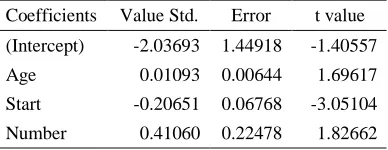
The results of logistic regression are given in Ta-ble 1.

Table 1: Logistic Regression Coefficients.

Coefficients Value Std. Error t value (Intercept) -2.03693 1.44918 -1.40557

Age 0.01093 0.00644 1.69617

Start -0.20651 0.06768 -3.05104 Number 0.41060 0.22478 1.82662

(Dispersion Parameter for Binomial family taken to be 1)

(3)

Table 1 reveals that all three covariates are statisti-cally significant and have expected directions. Ta-ble 2 shows the partial correlation between the co-variates.

Table 2: Correlation Matrix.

Age Start

Start -0.28495

Number 0.23210 0.11075

The coefficient standard errors reported by glm rely on asymptotic approximations and may not be trustworthy. Therefore, let us turn to the bootstrap. Here we want to fit a regression model with re-sponse variable

y

and predictors

x

₁

,

x

₂

,...

x

_k. We have a sample of n observations

)

,...,

,

(

₁ ₁ ₂

,

, i i ik

i

y

x

z

′

=

, i = 1, 2, …, n. Here we

simply select

B

bootstrap samples of the

z

_i

′

, fitting the model and saving the coefficients from each bootstrap sample.

We then construct confidence intervals for the re-gression coefficients using the methods discussed by Davidson and Hinkley (1997).

ORDINARY NONPARAMETRIC BOOTSTRAP

>boot.h

function(data, indices) { data <- data[indices, ]

mod <- glm(formula = Kyphosis ~ Age + Start + Number, family = binomial, data = data)

coefficients (mod) }

boot (data = kyphosis, statistic = boot.h, R = 999)

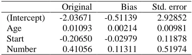
Table 3 shows the results of logistic regression performed from bootstrapping sample with a repli-cation of 999.

Table 3: Bootstrap Statistics for Selected Vari-ables.

Original Bias Std. error

(Intercept) -2.03671 -0.51139 2.92852

Age 0.01093 0.00214 0.00981

Start -0.20650 -0.02979 0.11878 Number 0.41056 0.11311 0.51974

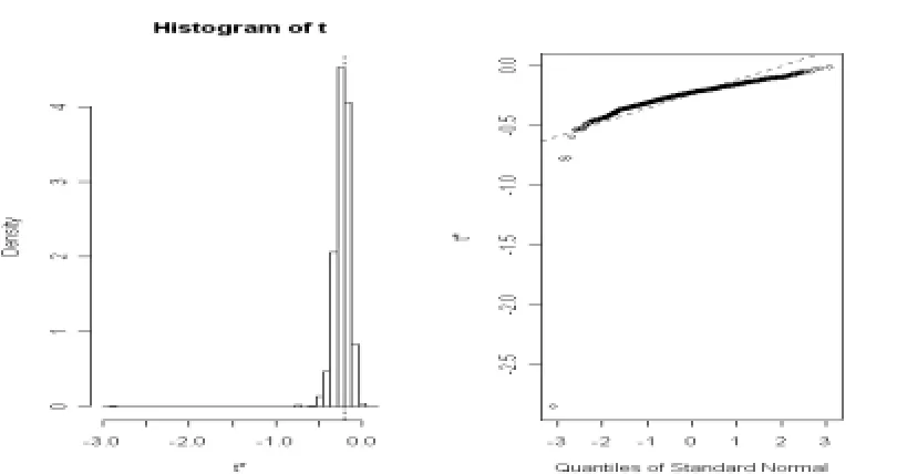
Figure 1-3 show the histograms and normal quan-tile-comparison plots for the bootstrap replications of the age (Figure 1), start (Figure 2) and number (figure 3) coefficients in Kyphosis data. The bro-ken vertical line in each histogram shows the loca-tion of the regression coefficient for the model to fit to the original sample.

While considering bootstrapping sample we find that except for Number, the bias is too small for covariates Age and Start. Looking at Figures 1-3, one can conclude that they follow approximately normal which in turn help us to justify the useful-ness of bootstrapping technique.

Tables 4 -9 show confidence intervals of coeffi-cients of logistic regression model. The confidence intervals are observed to be very close for covari-ates Age and Start; on the other hand, it is wider for Number. So the application of bootstrapping pro-vides us better understanding and better results.

> boot.ci (boot.out =boot.k,

type=c(“norm”,”prec”,bca”), index=2)

BOOTSTRAP CONFIDENCE INTERVAL CALCULATIONS

Based on 999 bootstrap replications

CALL :

Boot.ci (boot.out = boot.k, type=c (“norm”, “prec”, “bca”), index=2)

Table 4: 95% Confidence Intervals for Age.

(4)

Figure 2: Start Coefficient

(5)

CALL :

Boot.ci (boot.out = boot.k, conf = 0.9, type = c (“norm”, “prec”, “bca”), index=2)

Table 5: 90% Confidence Intervals for Age.

Level Normal Percentile BCa 90% -0.0073, 0.0249 0.0022, 0.0266 0.0005, 0.0225

boot.ci (boot.out = boot.k, type = c (“norm”, “prec”, “bca”), index=3)

Based on 999 bootstrap replicates

CALL :

boot.ci (boot.out = boot.k, type = c (“norm”, “prec”, “bca”), index=3)

Table 6: 95%Confidence Intervals for Start.

Level Normal Percentile BCa

95% -0.4095, 0.0561 -0.4337, -0.0969 -0.3507, -0.0454

boot.ci (boot.out = boot.k, conf = 0.9, type = c (“norm”, “prec”, “bca”), index=3)

Table 7: 90% Confidence Intervals for Start.

90% -0.3721, 0.0197 -0.3787, -0.1101 -0.3245, -0.0721

boot.ci (boot.out =boot.k, type=c(“norm”, ”prec”, ”bca”), index=4)

Based on 999 bootstrap replications

CALL :

Boot.ci (boot.out = boot.k, type=c (“norm”, “prec”, “bca”), index=4)

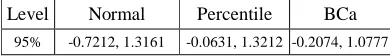
Table 8: 95% Confidence Intervals for Number.

95% -0.7212, 1.3161 -0.0631, 1.3212 -0.2074, 1.0777

CALL :

Boot.ci (boot.out = boot.k, conf = 0.9, type = c (“norm”, “prec”, “bca”), index=4)

Table 9: 90% Confidence Intervals for Number.

90% -0.5575, 1.1524 0.0250, 1.1509 -0.1313, 0.9366

The normal theory and percentile intervals are rea-sonably similar to each other, but the more trust-worthy

BC

_αintervals are somewhat different.

V. CONCLUSION

It may be concluded that the bootstrap method could potentially be applied to problems of statisti-cal error assessment beyond biases and standard errors, in particular to the setting of approximate confidence intervals, but only if further progress were made in understanding the bootstrap's inferen-tial biases.

VI. REFERENCES

1. A. C. Davidson, D.V. Hinkley: Bootstrap Methods and their Application. Cambridge: Cambridge University Press. (1997)

2. B. Efron: ``Bootstrap methods: another look at the Jackknife" Annals of Statistics, 7, pp 1-26. (1979)

3. B. Efron, R. J. Tibshirani: An Introduction to the Bootstrap. New York: Chapman and Hall. (1993)