Human Language Technologies: The 2009 Annual Conference of the North American Chapter of the ACL, pages 450–458,
Performance Prediction for Exponential Language Models
Stanley F. Chen
IBM T.J. Watson Research Center P.O. Box 218, Yorktown Heights, NY 10598
Abstract
We investigate the task of performance pre-diction for language models belonging to the exponential family. First, we attempt to em-pirically discover a formula for predicting test set cross-entropy for n-gram language mod-els. We build models over varying domains, data set sizes, andn-gram orders, and perform linear regression to see whether we can model test set performance as a simple function of training set performance and various model statistics. Remarkably, we find a simple rela-tionship that predicts test set performance with a correlation of 0.9997. We analyze why this relationship holds and show that it holds for other exponential language models as well, in-cluding class-based models and minimum dis-crimination information models. Finally, we discuss how this relationship can be applied to improve language model performance.
1 Introduction
In this paper, we investigate the following question for language models belonging to the exponential family: given some training data and test data drawn from the same distribution, can we accurately pre-dict the test set performance of a model estimated from the training data? This problem is known as performance prediction and is relevant for model se-lection, the task of selecting the best model from a set of candidate models given data.1
Let us first define some notation. Events have the form (x, y), where we attempt to predict the cur-rent wordygiven previous wordsx. We denote the training data asD= (x1, y1), . . . ,(xD, yD)and de-finep˜(x, y) = countD(x, y)/D to be the empirical distribution of the training data. Similarly, we have
1
A long version of this paper can be found at (Chen, 2008).
a test set D∗ and an associated empirical distribu-tionp∗(x, y). We take the performance of a condi-tional language modelp(y|x)to be the cross-entropy H(p∗, p) between the empirical test distribution p∗ and the modelp(y|x):
H(p∗, p) =−X
x,y
p∗(x, y) logp(y|x) (1)
This is equivalent to the negative mean log-likelihood per event, as well as to log perplexity.
We only consider models in the exponential fam-ily. An exponential modelpΛ(y|x)is a model with a set of features{f1(x, y), . . . , fF(x, y)}and equal number of parametersΛ ={λ1, . . . , λF}where
pΛ(y|x) =
exp(PFi=1λifi(x, y))
ZΛ(x)
(2)
and whereZΛ(x)is a normalization factor.
One of the seminal methods for performance pre-diction is the Akaike Information Criterion (AIC) (Akaike, 1973). For a model, let ˆΛ be the maxi-mum likelihood estimate ofΛon some training data. Akaike derived the following estimate for the ex-pected value of the test set cross-entropyH(p∗, pΛˆ):
H(p∗, pΛˆ)≈ H(˜p, pΛˆ) +
F
D (3)
H(˜p, pΛˆ) is the cross-entropy of the training set,F
is the number of parameters in the model, andDis the number of events in the training data. However, maximum likelihood estimates for language mod-els typically yield infinite cross-entropy on test data, and thus AIC behaves poorly for these domains.
In this work, instead of deriving a performance prediction relationship theoretically, we attempt to empirically discover a formula for predicting test performance. Initially, we consider onlyn-gram lan-guage models, and build models over varying do-mains, data set sizes, andn-gram orders. We per-form linear regression to discover whether we can
model test set cross-entropy as a simple function of training set cross-entropy and other model statistics. For the 200+n-gram models we evaluate, we find that the empirical relationship
H(p∗, pΛ˜)≈ H(˜p, pΛ˜) +
γ D
F X
i=1
|λ˜i| (4)
holds with a correlation of 0.9997 whereγis a con-stant and where˜Λ ={˜λi}are regularized parameter estimates; i.e., rather than estimating performance for maximum likelihood models as in AIC, we do this for regularized models. In other words, test set cross-entropy can be approximated by the sum of the training set cross-entropy and the scaled sum of the magnitudes of the model parameters.
To maximize the correlation achieved by eq. (4), we find that it is necessary to use the same regular-ization method and regularregular-ization hyperparameters across models and that the optimal value of γ de-pends on the values of the hyperparameters. Con-sequently, we first evaluate several types of regu-larization and find which of these (and which hy-perparameter values) work best across all domains, and use these values in all subsequent experiments. While`22 regularization gives the best performance reported in the literature forn-gram models, we find here that`1+`22regularization works even better.
The organization of this paper is as follows: In Section 2, we evaluate various regularization tech-niques forn-gram models and select the method and hyperparameter values that give the best overall per-formance. In Section 3, we discuss experiments to find a formula for predictingn-gram model perfor-mance, and provide an explanation for why eq. (4) works so well. In Section 4, we evaluate how well eq. (4) holds for several class-based language els and minimum discrimination information mod-els. Finally, in Sections 5 and 6 we discuss related work and conclusions.
2 Selecting Regularization Settings
In this section, we address the issue of how to per-form regularization in our later experiments. Fol-lowing the terminology of Dud´ık and Schapire (2006), the most widely-used and effective methods for regularizing exponential models are`1
regular-ization (Tibshirani, 1994; Kazama and Tsujii, 2003;
data token range training voc. source type ofn sents. size
A RH letter 2–7 100–75k 27
B WSJ POS 2–7 100–30k 45
C WSJ word 2–5 100–100k 300
D WSJ word 2–5 100–100k 3k
E WSJ word 2–5 100–100k 21k
F BN word 2–5 100–100k 84k
[image:2.612.325.532.61.169.2]G SWB word 2–5 100–100k 19k
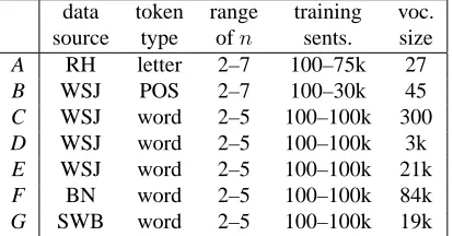
Table 1: Statistics of data sets. RH = Random House dictionary; WSJ = Wall Street Journal; BN = Broadcast News; SWB = Switchboard.
Goodman, 2004) and`22 regularization (Lau, 1994; Chen and Rosenfeld, 2000; Lebanon and Lafferty, 2001). While not as popular, another regularization scheme that has been shown to be effective is 2-norm inequality regularization (Kazama and Tsujii, 2003) which is an instance of`1+`2
2regularization as noted
by Dud´ık and Schapire (2006). Under`1+`22
regu-larization, the regularized parameter estimates˜Λare chosen to optimize the objective function
O`1+`22(Λ) =H(˜p, pΛ) +
α D
F X
i=1
|λi|+
1 2σ2D
F X
i=1
λ2i
(5)
Note that`1regularization can be considered a
spe-cial case of this (by takingσ = ∞) as can`22 regu-larization (by takingα= 0).
Here, we evaluate`1,`22, and`1+`22
regulariza-tion for exponential n-gram models. An exponen-tialn-gram model contains a binary featurefω for each n0-gram ω occurring in the training data for n0 ≤ n, wherefω(x, y) = 1 iffxy ends inω. We would like to find the regularization method and as-sociated hyperparameters that work best across dif-ferent domains, training set sizes, and n-gram or-ders. As it is computationally expensive to evalu-ate a large number of hyperparameter settings over a large collection of models, we divide this search into two phases. First, we evaluate a large set of hy-perparameters on a limited set of models to come up with a short list of candidate hyperparameters. We then evaluate these candidates on our full model set to find the best one.
in total. We refer to these domains by the letters A– G; summary statistics for each domain are given in Table 1. The domains C–G consist of regular word data, while domains A and B consist of letter and part-of-speech (POS) sequences, respectively. Do-mains C–E differ only in vocabulary.
[image:3.612.352.501.57.248.2]For each domain, we first randomize the order of sentences in that data. We partition off two devel-opment sets and an evaluation set (5000 “sentences” each in domain A and 2500 sentences elsewhere) and use the remaining data as training data. In this way, we assure that our training and test data are drawn from the same distribution as is assumed in our later experiments. Training set sizes in sentences are 100, 300, 1000, 3000, etc., up to the maximums given in Table 1. Building models for each training set size andn-gram order in Table 1 gives us a total of 218 models over the seven domains.
In the first phase of hyperparameter search, we choose a subset of these models (57 total) and evalu-ate many different values for(α, σ2)with`1+`22 reg-ularization on each. We perform a grid search, trying each value α ∈ {0.0,0.1,0.2, . . . ,1.2} with each valueσ2∈ {1,1.2,1.5,2,2.5,3,4,5,6,7,8,10,∞} whereσ =∞ corresponds to`1 regularization and
α = 0 corresponds to `2
2 regularization. We use
a variant of iterative scaling for parameter estima-tion. For each model and each(α, σ2), we denote the cross-entropy of the development data asHm
α,σ for themth model,m∈ {1, . . . ,57}. Then, for each mand(α, σ2), we can compute how much worse the settings(α, σ2)perform with modelmas compared
to the best hyperparameter settings for that model:
ˆ
Hα,σm =Hα,σm −min α0,σ0H
m
α0,σ0 (6)
We would like to select(α, σ2)for whichHˆα,σm tends to be small; in particular, we choose (α, σ2) that
minimizes the root mean squared (RMS) error
ˆ
Hα,σRMS= v u u
t1
57
57 X
m=1
( ˆHm
α,σ)2 (7)
For each of`1,`22, and`1+`22regularization, we
re-tain the 6–8 best hyperparameter settings. To choose the best single hyperparameter setting from within this candidate set, we repeat the same analysis ex-cept over the full set of 218 models.
statistic RMSE coeff.
1 D
PF
i=1|˜λi| 0.043 0.938 1
D P
i:˜λi>0λ˜i 0.044 0.939 1
D PF
i=1˜λi 0.047 0.940 1
D PF
i=1|λ˜i| 4
3 0.162 0.755 1
D PF
i=1|λ˜i| 3
2 0.234 0.669 1
D PF
i=1λ˜2i 0.429 0.443 F6=0
D 0.709 1.289
F6=0logD
D 0.783 0.129
F
D 0.910 1.109
FlogD
D 0.952 0.112
1 1.487 1.698
F
D−F−1 2.232 -0.028 F6=0
D−F6=0−1 2.236 -0.023
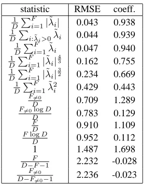
Table 2: Root mean squared error (RMSE) in nats when predicting difference in development set and training set cross-entropy as linear function of a single statistic. The last column is the optimal coefficient for that statistic.
On the development sets, the (α, σ2) value with the lowest squared error is (0.5, 6), and these are the hyperparameter settings we use in all later ex-periments unless otherwise noted. The RMS error, mean error, and maximum error for these hyperpa-rameters on the evaluation sets are 0.011, 0.007, and 0.033 nats, respectively.2An error of 0.011 nats cor-responds to a 1.1% difference in perplexity which is generally considered insignificant. Thus, we can achieve good performance across domains, data set sizes, andn-gram orders using a single set of hyper-parameters as compared to optimizing hyperparam-eters separately for each model.
3 N-Gram Model Performance Prediction
Now that we have established which regularization method and hyperparameters to use, we attempt to empirically discover a simple formula for predict-ing the test set cross-entropy of regularizedn-gram models. The basic strategy is as follows: We first build a large number ofn-gram models over differ-ent domains, training set sizes, andn-gram orders. Then, we come up with a set of candidate statistics, e.g., training set cross-entropy, number of features, etc., and do linear regression to try to best model test
2
0 1 2 3 4 5 6 7
0 1 2 3 4 5 6 7
test cross-entropy - training cross-entropy (nats)
∑ |λi| / D
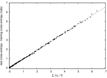
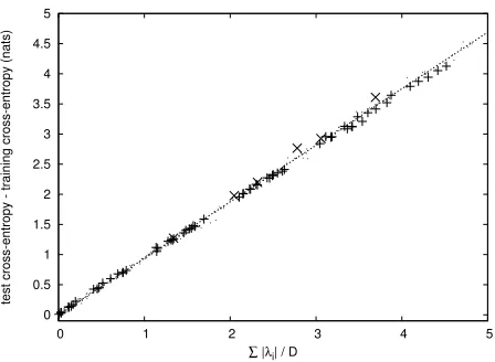
Figure 1: Graph of optimism on evaluation data vs.
1 D
PF
i=1|˜λi| for variousn-gram models under `1 +`22
regularization, α = 0.5 andσ2 = 6. The line
repre-sents the predicted optimism according to eq. (9) with
γ= 0.938.
set cross-entropy as a linear function of these statis-tics. We assume that training and test data come from the same distribution; otherwise, it would be difficult to predict test performance.
We use the same 218 n-gram models as in Sec-tion 2. For each model, we compute training set cross-entropy H(˜p, pΛ˜) as well as all of the
statis-tics listed on the left in Table 2. The statisstatis-tics FD, F
D−F−1, and
FlogD
D are motivated by AIC, AICc (Hurvich and Tsai, 1989), and the Bayesian Infor-mation Criterion (Schwarz, 1978), respectively. As features fi with ˜λi = 0 have no effect, instead of
F we also consider using F6=0, the number of
fea-turesfiwithλ˜i 6= 0. The statistics D1 PFi=1|λ˜i|and 1
D
PF
i=1λ˜2i are motivated by eq. (5). The statistics with fractional exponents are suggested by Figure 2. The value 1 is present to handle constant offsets.
After some initial investigation, it became clear that training set cross-entropy is a very good (par-tial) predictor of test set cross-entropy with coeffi-cient 1. As there is ample theoretical support for this, instead of fitting test set performance directly, we chose to model the difference between test and training performance as a function of the remaining statistics. This difference is sometimes referred to as the optimism of a model:
optimism(pΛ˜)≡ H(p∗, pΛ˜)− H(˜p, pΛ˜) (8)
First, we attempt to model optimism as a lin-ear function of a single statistic. For each statis-tic listed previously, we perform linear regression to minimize root mean squared error when predict-ing development set optimism. In Table 2, we dis-play the RMSE and best coefficient for each statis-tic. We see that three statistics have by far the lowest error: D1 PFi=1|˜λi|, D1 Pi:˜λi>0˜λi, and D1 PFi=1λ˜i. In practice, mostλ˜i inn-gram models are positive, so these statistics tend to have similar values. We choose the best ranked of these, D1 PFi=1|˜λi|, and show in Section 3.1 why this statistic is more appeal-ing than the others. Next, we investigate modelappeal-ing optimism as a linear function of a pair of statistics. We find that the best RMSE for two variables (0.042) is only slightly lower than that for one (0.043), so it is doubtful that a second variable helps.
Thus, our analysis suggests that among our candi-dates, the best predictor of optimism is simply
optimism≈ γ
D
F X
i=1
|˜λi| (9)
whereγ = 0.938, with this value being independent of domain, training set size, andn-gram order. In other words, the difference between test and train-ing cross-entropy is a linear function of the sum of parameter magnitudes scaled per event. Substituting into eq. (8) and rearranging, we get eq. (4).
To assess the accuracy of eq. (4), we compute var-ious statistics on our evaluation sets using the best γ from our development data, i.e., γ = 0.938. In Figure 1, we graph optimism for the evaluation data against D1 PFi=1|λ˜i|for each of our models; we see that the linear correlation is very good. The correla-tion between the actual and predicted cross-entropy on the evaluation data is 0.9997; the mean absolute prediction error is 0.030 nats; the RMSE is 0.043 nats; and the maximum absolute error is 0.166 nats. Thus, on average we can predict test performance to within 3% in perplexity, though in the worst case we may be off by as much as 18%.3
3
[image:4.612.75.299.57.222.2]empiri--1.5 -1 -0.5 0 0.5 1 1.5 2 2.5
-1 0 1 2 3 4
discount
[image:5.612.72.297.58.219.2]λ
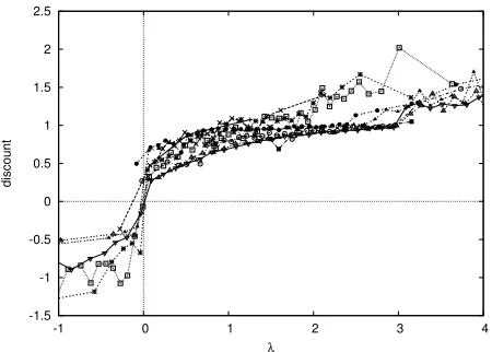
Figure 2: Smoothed graph of discount versusλ˜i for all
features in ten different models built on domains A and
E. Each smoothed point represents the average of at least
512 raw data points.
If we compute the prediction error of eq. (4) over the same models except using `1 or`22
regulariza-tion (with the best corresponding hyperparameter values found in Section 2), the prediction RMSE is 0.054 and 0.139 nats, respectively. Thus, we find that choosing hyperparameters carefully in Section 2 was important in doing well in performance predic-tion. While hyperparameters were chosen to opti-mize test performance rather than prediction accu-racy, we find that the chosen hyperparameters are favorable for the latter task as well.
3.1 Why Does Prediction Work So Well?
The correlation in Figure 1 is remarkably high, and thus it begs for an explanation. First, let us express the difference in test and training cross-entropy for a model in terms of its parametersΛ. Substituting eq. (2) into eq. (1), we get
H(p∗, pΛ) =− F X
i=1
λiEp∗[fi] + X
x
p∗(x) logZΛ(x)
(10)
where Ep∗[fi] = Px,yp∗(x, y)fi(x, y). Then, we
can express the difference in test and training per-formance as
H(p∗, p
Λ)− H(˜p, pΛ) =PFi=1λi(Ep˜[fi]−Ep∗[fi])+
P
x(p∗(x)−p˜(x)) logZΛ(x) (11)
cal standard deviation across test sets was found to be 0.0123, 0.0144, 0.0167, and 0.0174 nats, respectively. This effect can be mitigated by simply using larger test sets.
Ignoring the last term on the right, we see that opti-mism for exponential models is a linear function of theλi’s with coefficientsEp˜[fi]−Ep∗[fi].
Then, we can ask what Ep˜[fi]−Ep∗[fi] values would let us satisfy eq. (4). Consider the relationship
(Ep˜[fi]−Ep∗[fi])×D≈γsgnλ˜i (12)
If we substitute this into eq. (11) and ignore the last term on the right again, this gives us exactly eq. (4). We refer to the value(Ep˜[fi]−Ep∗[fi])×Das the discount of a feature. It can be thought of as rep-resenting how many times less the feature occurs in the test data as opposed to the training data, if the test data were normalized to be the same size as the training data. Discounts forn-grams have been stud-ied extensively, e.g., (Good, 1953; Church and Gale, 1991; Chen and Goodman, 1998), and tend not to vary much across training set sizes.
We can check how well eq. (12) holds for actual regularizedn-gram models. We construct a total of tenn-gram models on domains A and E. We build four letter 5-gram models on domain A on training sets ranging in size from 100 words to 30k words, and six models (either trigram or 5-gram) on do-main E on training sets ranging from 100 sentences to 30k sentences. We create large development test sets (45k words for domain A and 70k sentences for domain E) to better estimateEp∗[fi].
Because graphs of discounts as a function of λ˜i are very noisy, we smooth the data before plotting. We partition data points into buckets containing at least 512 points. We average all of the points in each bucket to get a “smoothed” data point, and plot this single point for each bucket. In Figure 2, we plot smoothed discounts as a function of˜λiover the rangeλ˜i∈[−1,4]for all ten models.
We see that eq. (12) holds at a very rough level over the λ˜i range displayed. If we examine how much different ranges of ˜λi contribute to the over-all value ofPFi=1λ˜i(Ep˜[fi]−Ep∗[fi]), we find that the great majority of the mass (90–95%+) is concen-trated in the rangeλ˜i ∈[0,4]for all ten models un-der consiun-deration. Thus, to a first approximation, the reason that eq. (4) holds withγ = 0.938is because on average, feature expectations have a discount of about this value forλ˜iin this range.4
4
0 0.5 1 1.5 2 2.5 3 3.5 4 4.5 5
0 1 2 3 4 5
test cross-entropy - training cross-entropy (nats)
∑ |λi| / D
Figure 3: Graph of optimism on evaluation data vs.
1 D
PF
i=1|˜λi| for various models. The ‘+’ marks
corre-spond to models S, M, and L over different training set sizes,n-gram orders, and numbers of classes. The ‘×’ marks correspond to MDI models over differentn-gram orders and in-domain training set sizes. The line and small points are taken from Figure 1.
Due to space considerations, we only summarize our other findings; a longer discussion is provided in (Chen, 2008). We find that the absolute error in cross-entropy tends to be quite small across models for several reasons. For non-sparse models, there is significant variation in average discounts, but be-cause D1 PFi=1|λ˜i| is low, the overall error is low. In contrast, sparse models are dominated by single-countn-grams with features whose average discount is quite close toγ = 0.938. Finally, the last term on the right in eq. (11) also plays a small but significant role in keeping the prediction error low.
4 Other Exponential Language Models
In (Chen, 2009), we show how eq. (4) can be used to motivate a novel class-based language model and a regularized version of minimum discrimination in-formation (MDI) models (Della Pietra et al., 1992). In this section, we analyze whether in addition to word n-gram models, eq. (4) holds for these other exponential language models as well.
won’t hold. For example, if a feature functionfiis doubled, its
expectations and discount will also double. Thus, eq. (4) won’t hold in general for models with continuous feature values, as average discounts may vary widely.
4.1 Class-Based Language Models
We assume a wordwis always mapped to the same classc(w). For a sentencew1· · ·wl, we have
p(w1· · ·wl) =Ql+1j=1p(cj|c1· · ·cj−1, w1· · ·wj−1)× Ql
j=1p(wj|c1· · ·cj, w1· · ·wj−1) (13)
where cj = c(wj) and where cl+1 is an
end-of-sentence token. We use the notation png(y|ω) to
denote an exponentialn-gram model as defined in Section 2, where we have features for each suffix of each ωy occurring in the training set. We use the notationpng(y|ω1, ω2)to denote a model containing
all features in the modelspng(y|ω1)andpng(y|ω2).
We consider three class models, models S, M, and
L, defined as
pS(cj|c1···cj−1,w1···wj−1)=png(cj|cj−2cj−1)
pS(wj|c1···cj,w1···wj−1)=png(wj|cj)
pM(cj|c1···cj−1,w1···wj−1)=png(cj|cj−2cj−1,wj−2wj−1)
pM(wj|c1···cj,w1···wj−1)=png(wj|wj−2wj−1cj)
pL(cj|c1···cj−1,w1···wj−1)=png(cj|wj−2cj−2wj−1cj−1)
pL(wj|c1···cj,w1···wj−1)=png(wj|wj−2cj−2wj−1cj−1cj)
Model S is an exponential version of the class-based n-gram model from (Brown et al., 1992); model M is a novel model introduced in (Chen, 2009); and model L is an exponential version of the model ind-expredict from (Goodman, 2001).
To evaluate whether eq. (4) can accurately pre-dict test performance for these class-based models, we use the WSJ data and vocabulary from domain E and consider training set sizes of 1k, 10k, 100k, and 900k sentences. We create three different word classings containing 50, 150, and 500 classes using the algorithm of Brown et al. (1992) on the largest training set. For each training set and number of classes, we build both 3-gram and 4-gram versions of each of our three class models.
[image:6.612.75.299.57.221.2]class n-gram models using the same γ = 0.938 value found for wordn-gram models. The mean ab-solute prediction error is 0.029 nats, comparable to that found for wordn-gram models.
It is interesting that eq. (4) works for class-based models despite their being composed of two sub-models, one for word prediction and one for class prediction. However, taking the log of eq. (13), we note that the cross-entropy of text can be expressed as the sum of the cross-entropy of its word tokens and the cross-entropy of its class tokens. It would not be surprising if eq. (4) holds separately for the class prediction model predicting class data and the word prediction model predicting word data, since all of these component models are basicallyn-gram models. Summing, this explains why eq. (4) holds for the whole class model.
4.2 Models with Prior Distributions
Minimum discrimination information models (Della Pietra et al., 1992) are exponential models with a prior distributionq(y|x):
pΛ(y|x) =q(y|x)
exp(PFi=1λifi(x, y))
ZΛ(x)
(14)
The central issue in performance prediction for MDI models is whetherq(y|x)needs to be accounted for. That is, if we assume q is an exponential model, should its parametersλqi be included in the sum in eq. (4)? From eq. (11), we note that if Ep˜[fi]−
Ep∗[fi] = 0 for a featurefi, then the feature does
not affect the difference between test and training cross-entropy (ignoring its impact on the last term). By assumption, the training and test set forpcome from the same distribution while q is derived from an independent data set. It follows that we expect Ep˜[fiq]−Ep∗[fiq]to be zero for features inq, and we
should ignoreqwhen applying eq. (4).
To evaluate whether eq. (4) holds for MDI mod-els, we use the same WSJ training and evaluation sets from domain E as in Section 4.1. We consider three different training set sizes: 1k, 10k, and 100k sentences. To trainq, we use the 100k sentence BN training set from domain F. We build both trigram and 4-gram versions of each model.
In Figure 3, we plot test minus training cross-entropy versus D1 PFi=1|λ˜i|for these models on our WSJ evaluation set; the ‘×’ marks correspond to
the MDI models. As expected, eq. (4) appears to work quite well for MDI models using the same γ = 0.938value as before; the mean absolute pre-diction error is 0.077 nats.
5 Related Work
We group existing performance prediction methods into two categories: non-data-splitting methods and data-splitting methods. In non-data-splitting meth-ods, test performance is directly estimated from training set performance and/or other statistics of a model. Data-splitting methods involve partitioning training data into a truncated training set and a surro-gate test set and using surrosurro-gate test set performance to estimate true performance.
The most popular non-data-splitting methods for predicting test set cross-entropy (or likelihood) are AIC and variants such as AICc, quasi-AIC (QAIC), and QAICc(Akaike, 1973; Hurvich and Tsai, 1989; Lebreton et al., 1992). In Section 3, we consid-ered performance prediction formulae with the same form as AIC and AICc(except using regularized pa-rameter estimates), and neither performed as well as eq. (4); e.g., see Table 2.
There are many techniques for bounding test set classification error including the Occam’s Ra-zor bound (Blumer et al., 1987; McAllester, 1999), PAC-Bayes bound (McAllester, 1999), and the sam-ple compression bound (Littlestone and Warmuth, 1986; Floyd and Warmuth, 1995). These methods derive theoretical guarantees that the true error rate of a classifier will be below (or above) some value with a certain probability. Langford (2005) evalu-ates these techniques over many data sets; while the bounds can sometimes be fairly tight, in many data sets the bounds are quite loose.
In practice, the most accurate methods for perfor-mance prediction in many contexts are data-splitting methods (Guyon et al., 2006). These techniques in-clude the hold-out method; leave-one-out andk-fold cross-validation; and bootstrapping (Allen, 1974; Stone, 1974; Geisser, 1975; Craven and Wahba, 1979; Efron, 1983). However, unlike non-data-splitting methods, these methods do not lend them-selves well to providing insight into model design as discussed in Section 6.
6 Discussion
We show that for several types of exponential lan-guage models, it is possible to accurately predict the cross-entropy of test data using the simple relation-ship given in eq. (4). When using`1+`22
regulariza-tion with(α = 0.5, σ2 = 6), the valueγ = 0.938 works well across varying model types, domains, vocabulary sizes, training set sizes, andn-gram or-ders, yielding a mean absolute error of about 0.03 nats (3% in perplexity). We evaluate∼300 language models in total, including word and class n-gram models andn-gram models with prior distributions. While there has been a great deal of work in performance prediction, the vast majority of work on non-data-splitting methods has focused on find-ing theoretically-motivated approximations or prob-abilistic bounds on test performance. In contrast, we developed eq. (4) on a purely empirical basis, and there has been little, if any, existing work that has shown comparable performance prediction accuracy over such a large number of models and data sets. In addition, there has been little, if any, previous work on performance prediction for language modeling.5
While eq. (4) performs well as compared to other non-data-splitting methods for performance predic-tion, the prediction error can be several percent in perplexity, which means we cannot reliably rank models that are close in quality. In addition, in speech recognition and many other applications, an external test set is typically provided, which means we can measure test set performance directly. Thus, in practice, eq. (4) is not terribly useful for the task
5
Here, we refer to predicting test set performance from training set performance and other model statistics. However, there has been a good deal of work on predicting speech recog-nition word-error rate from test set perplexity and other statis-tics, e.g., (Klakow and Peters, 2002).
of model selection; instead, what eq. (4) gives us is insight into model design. That is, instead of select-ing between candidate models once they have been built as in model selection, it is desirable to be able to select between models at the model design stage. Being able to intelligently compare models (with-out implementation) requires that we know which aspects of a model impact test performance, and this is exactly what eq. (4) tells us.
Intuitively, simpler models should perform better on test data given equivalent training performance, and model structure (as opposed to parameter val-ues) is an important aspect of the complexity of a model. Accordingly, there have been many meth-ods for model selection that measure the size of a model in terms of the number of features or param-eters in the model, e.g., (Akaike, 1973; Rissanen, 1978; Schwarz, 1978). Surprisingly, for exponential language models, the number of model parameters seems to matter not at all; all that matters are the magnitudes of the parameter values. Consequently, one can improve such models by adding features (or a prior model) that reduce parameter values while maintaining training performance.
In (Chen, 2009), we show how these ideas can be used to motivate heuristics for improving the perfor-mance of existing language models, and use these heuristics to develop a novel class-based model and a regularized version of MDI models that outper-form comparable methods in both perplexity and speech recognition word-error rate on WSJ data. In addition, we show how the tradeoff between train-ing set performance and model size impacts aspects of language modeling as diverse as backoffn-gram features, class-based models, and domain adapta-tion. In sum, eq. (4) provides a new and valuable framework for characterizing, analyzing, and de-signing statistical models.
Acknowledgements
We thank Bhuvana Ramabhadran and the anony-mous reviewers for their comments on this and ear-lier versions of the paper.
References
Sec-ond Intl. Symp. on Information Theory, pp. 267–281.
David M. Allen. 1974. The relationship between vari-able selection and data augmentation and a method for prediction. Technometrics, 16(1):125–127.
Peter L. Bartlett. 1998. The sample complexity of pat-tern classification with neural networks: the size of the weights is more important than the size of the network.
IEEE Trans. on Information Theory, 44(2):525–536.
Alselm Blumer, Andrzej Ehrenfeucht, David Haussler, and Manfred K. Warmuth. 1987. Occam’s razor.
In-formation Processing Letters, 24(6):377–380.
Peter F. Brown, Vincent J. Della Pietra, Peter V. deSouza, Jennifer C. Lai, and Robert L. Mercer. 1992. Class-based n-gram models of natural language.
Computa-tional Linguistics, 18(4):467–479, December.
Stanley F. Chen and Joshua Goodman. 1998. An empir-ical study of smoothing techniques for language mod-eling. Tech. Report TR-10-98, Harvard Univ.
Stanley F. Chen and Ronald Rosenfeld. 2000. A survey of smoothing techniques for maximum entropy mod-els. IEEE Trans. Speech and Aud. Proc., 8(1):37–50. Stanley F. Chen. 2008. Performance prediction for
ex-ponential language models. Tech. Report RC 24671, IBM Research Division, October.
Stanley F. Chen. 2009. Shrinking exponential language models. In Proc. of HLT-NAACL.
Kenneth W. Church and William A. Gale. 1991. A com-parison of the enhanced Good-Turing and deleted esti-mation methods for estimating probabilities of English bigrams. Computer Speech and Language, 5:19–54. Peter Craven and Grace Wahba. 1979. Smoothing noisy
data with spline functions: estimating the correct de-gree of smoothing by the method of generalized cross-validation. Numerische Mathematik, 31:377–403. Stephen Della Pietra, Vincent Della Pietra, Robert L.
Mercer, and Salim Roukos. 1992. Adaptive language modeling using minimum discriminant estimation. In
Proc. Speech and Natural Lang. DARPA Workshop.
Miroslav Dud´ık and Robert E. Schapire. 2006. Maxi-mum entropy distribution estimation with generalized regularization. In Proc. of COLT.
Bradley Efron. 1983. Estimating the error rate of a pre-diction rule: Improvement on cross-validation. J. of
the American Statistical Assoc., 78(382):316–331.
Sally Floyd and Manfred Warmuth. 1995. Sample com-pression, learnability, and the Vapnik-Chervonenkis dimension. Machine Learning, 21(3):269–304. Seymour Geisser. 1975. The predictive sample reuse
method with applications. J. of the American
Statisti-cal Assoc., 70:320–328.
I.J. Good. 1953. The population frequencies of species and the estimation of population parameters.
Biometrika, 40(3 and 4):237–264.
Joshua T. Goodman. 2001. A bit of progress in language modeling. MSR-TR-2001-72, Microsoft Research. Joshua Goodman. 2004. Exponential priors for
maxi-mum entropy models. In Proc. of NAACL.
Isabelle Guyon, Amir Saffari, Gideon Dror, and Joachim Buhmann. 2006. Performance prediction challenge. In Proc. of Intl. Conference on Neural Networks
(IJCNN06), IEEE World Congress on Computational Intelligence (WCCI06), pp. 2958–2965, July.
Clifford M. Hurvich and Chih-Ling Tsai. 1989. Regres-sion and time series model selection in small samples.
Biometrika, 76(2):297–307, June.
Jun’ichi Kazama and Jun’ichi Tsujii. 2003. Evaluation and extension of maximum entropy models with in-equality constraints. In Proc. of EMNLP, pp. 137–144. Dietrich Klakow and Jochen Peters. 2002. Testing the correlation of word error rate and perplexity. Speech
Communications, 38(1):19–28.
John Langford. 2005. Tutorial on practical prediction theory for classification. J. of Machine Learning
Re-search, 6:273–306.
Raymond Lau. 1994. Adaptive statistical language mod-elling. Master’s thesis, Department of Electrical En-gineering and Computer Science, Massachusetts Insti-tute of Technology, Cambridge, MA.
Guy Lebanon and John Lafferty. 2001. Boosting and maximum likelihood for exponential models. Tech. Report CMU-CS-01-144, Carnegie Mellon Univ. Jean-Dominique Lebreton, Kenneth P. Burnham, Jean
Clobert, and David R. Anderson. 1992. Modeling sur-vival and testing biological hypotheses using marked animals: a unified approach with case studies.
Eco-logical Monographs, 62:67–118.
Nick Littlestone and Manfred K. Warmuth. 1986. Re-lating data compression and learnability. Tech. report, Univ. of California, Santa Cruz.
David A. McAllester. 1999. PAC-Bayesian model aver-aging. In Proc. of COLT, pp. 164–170.
Jorma Rissanen. 1978. Modeling by the shortest data description. Automatica, 14:465–471.
Gideon Schwarz. 1978. Estimating the dimension of a model. Annals of Statistics, 6(2):461–464.
M. Stone. 1974. Cross-validatory choice and assessment of statistical predictions. J. of the Royal Statistical
So-ciety B, 36:111–147.
Robert Tibshirani. 1994. Regression shrinkage and se-lection via the lasso. Tech. report, Univ. of Toronto. Vladimir N. Vapnik. 1998. Statistical Learning Theory.