The British Binary Option

https://www.scirp.org/journal/jmf ISSN Online: 2162-2442

ISSN Print: 2162-2434

DOI: 10.4236/jmf.2019.94038 Nov. 14, 2019 747 Journal of Mathematical Finance

The British Binary Option

Min Gao1,2

1_{Sun Yat-Sen Business School, Guangzhou, China} 2_{Huafa Induatrial Share Co., LTD., Zhuhai, China}

Abstract

Following the economic rationale of the British options, we present a new class of binary options where the holder enjoys the early exercise feature of the American binary options with his payoff is the “best prediction” of the European binary payoff under the hypothesis that the true drift equals a con-tract drift. Based on the observed price movements, the option holder finds that the true drift of the stock price is unfavourable then he can substitute it with the contract drift. The key to the British binary option is the protection feature and to minimize the losses. A closed form expression for the arbi-trage-free price is derived in terms of the rational exercise boundary and the rational exercise boundary itself can be characterized as the unique solution to a nonlinear integral equation. We also analyze the financial meaning of the British binary options using the results above.

Keywords

British Binary Option, American Binary Option, Arbitrage-Free Price, Rational Exercise Boundary, Optimal Stopping, Geometric Brownian Motion, Parabolic Free Boundary Problem

1. Introduction

The purpose of the present paper is to introduce and examine the British payoff mechanism (see [1] and [2]) in the context of binary options. The main idea of the “British” feature provides the option holder a protection mechanism against unfavourable stock price movements. The contract buyer is able to substitute the true drift with a contract drift to make his payoff the best prediction of the Eu-ropean binary payoff.

Following the economic rationale of [1] and [2], we introduce a new binary op-tion that endogenously provides its holder with a protecop-tion mechanism against unfavourable stock price movements. This protection feature is intrinsically built How to cite this paper: Gao, M. (2019)

The British Binary Option. Journal of Ma-thematical Finance, 9, 747-762.

https://doi.org/10.4236/jmf.2019.94038

Received: June 6, 2019 Accepted: November 11, 2019 Published: November 14, 2019

Copyright © 2019 by author(s) and Scientific Research Publishing Inc. This work is licensed under the Creative Commons Attribution International License (CC BY 4.0).

http://creativecommons.org/licenses/by/4.0/

DOI: 10.4236/jmf.2019.94038 748 Journal of Mathematical Finance into the option contract and we refer to such contracts as “British” for the rea-sons outlined in [1] and [2]. The British binary option not only provides a unique protection against unfavourable stock price movements (see more details in Section 5) but also enables the option holder to obtain high returns when the stock price movements are favourable in both liquid and illiquid markets. It is useful to recall the notion “compound option” by Geske where an analytical so-lution for compound options was derived (see [3] and references therein). We refer to a more recent paper [4] for an informative review. This notion is also used in [5] [6] [7] [8] and [9] for the value of British Asian, British Russian and British lookback options. The arbitrage-free price of the option is a solution to an optimal stopping problem with the gain function as the payoff of the option (see [10]). We use a local time-space calculus on curves (see [11]) to derive a closed form expression for the arbitrage-free price in terms of the optimal stop-ping boundary and show that the free boundary itself is a unique solution to a nonlinear integral equation.

The paper is organized as follows. In Section 2 we present a basic motivation for the British cash-or-nothing put option. In Section 3 we first formally define the British cash-or-nothing put option and present some of its basic properties. We continue in Section 4 to derive a closed form expression for the arbi-trage-free price in terms of the rational exercise boundary and show that the ra-tional exercise boundary can be characterized as the unique solution to a nonli-near integral equation. In Section 5 we provide a financial analysis using the re-sults above (making comparisons with American binary options). In the final section, we present other different types of binary options: 1) calls or puts; 2) cash-or-nothing or asset-or-nothing.

2. Basic Motivation for the British Binary Option

The basic economic motivation for the British binary option is parallel to that of British put and call options (see [1] and [2]). In this section, we briefly review the key elements of the motivation on the cash-or-nothing put option.

1) Consider the stock price X and a riskless bond B evolving respectively as:

dXt=µX ttd +σX Wtd t (1)

dBt =rB ttd (2)

with X0=x and B0 =1 where µ∈R is the drift, σ >0 is the volatility coefficient, W =

( )

Wt t≥0 denotes the standard Brownian motion on a probabili-ty space

(

Ω,, P

)

and r>0 is the interest rate. The European or American put option is well defined in the literature (see [12]). Based on self-financing portfolios it implies that the arbitrage-free price of the options is given by (see [13]):

(

)

Q

E e rT T

V = _ − I X <K _ (European cash-or-nothing put option) (3)

(

)

Q

0

sup E e r T

V τI Xτ K

τ

− ≤ ≤

 

DOI: 10.4236/jmf.2019.94038 749 Journal of Mathematical Finance where the expectation Q

E is taken with respect to the unique equivalent

mar-tingale measure Q (see [10]) and the supremum is taken over all stopping times τ of X with values in

[ ]

0,T .

2) Recall that the arbitrage-free price for a European cash-or-nothing put op-tion is given by

(

)

(

)

Q

E e rT T

V = − I X <K (5)

where the expectation _EQ _{is taken with respect to the unique equivalent} mar-tingale measure Q. From the stochastic differential Equation (1), we get the unique strong solution

( )

(

(

2

)

)

exp 2

t t

X µ =x σW + µ σ− t (6)

under P for t∈

[ ]

0,T . We see that µ→Xt

( )

µ is strictly increasing so that

(

)

e rTI XT K

µ_→ − _<

is decreasing on R. Furthermore, it is well known that

( )

(

)

Law X µ | Q is the same as Law

(

X r

( )

| P

)

. Therefore, if µ=r we get

( )

(

)

(

)

E e rTI T .

V = − X µ <K (7)

The left-hand side stands for the value of investment and the right-hand side represents the expected value of the payoff. On the other hand, the option holder is glad to see µ<r. It follows

( )

(

)

(

)

E erTI T .

V < − X µ <K (8)

Then we say the return is “favourable”. On the contrary the return is “unfavourable” if µ>r and

( )

(

)

(

)

E e rTI .

T

V > − X µ <K (9)

3) In the real financial market, the actual drift µ is unknown at time t=0 and is not easy to estimate at later times t∈

(

0,T

]

in finite horizon. One will

buy the option if he believes that µ<r and surely he is pleased to see what

DOI: 10.4236/jmf.2019.94038 750 Journal of Mathematical Finance 4) In a real financial market, true buyer’s ability to sell will be determined by the market and this may also involve additional transaction costs and/or taxes. By “true buyer” we mean a buyer who has no ability or desire to sell the option at T in the European case or at the optimal stopping time τ in the American case. Furthermore, in most practical situations of over-the-counter trading it may be increasingly difficult to sell the option when out-of-money and makes the option expire worthless. Also in the real world the liquidity of the option market varies with the term of the contract, for example some extreme news event may lead to the option contract to become worthless once the news is re-leased. On the other hand, the protection feature endogenously built into the British option protect the option holder regardless of whether the option market is liquid or not.

3. The British Cash-or-Nothing Put Option: Definition and

Basic Properties

We start this section from a definition of the British cash-or-nothing put option and then give a brief analysis of its properties and rational exercise strategy.

Definition 1 The British cash-or-nothing put option is a financial contract between a seller/hedger and a buyer/holder entitling the latter to exercise at any (stopping) time τ _{prior to T whereupon his payoff is the “best prediction” of} the European cash-or-nothing payoff I X

(

T <K

)

given all the information up to time τ _{under the hypothesis that the true drift of the stock price equals} µc.

We refer µc as “contract drift” and it is natural that µc satisfies

.

c r

µ > ₍₁₀₎

if µc≤r the put option holder will beat the interest rate r by exercising imme-diately. Furthermore, µc can be as large as ∞, which means the option hold-er’s infinite tolerance for the true drift. Meanwhile the British cash-or-nothing put option would become a European cash-or-nothing put option.

1) We define the payoff function _Gµc as

(

,

)

E I

(

)

|

c c

t T t

Gµ t X = µ _ X <K _ (11)

where the conditional expectation is taken with respect to a new probability measure Pµc under which the stock price X expressed as

dXt =µcX ttd +σX Wtd t. (12)

We see from (1) and (12) that if we exercise the British option, the true (un-known) drift is substituted by the contract drift. Such a contract is referred as “British” since in terms of payoff the British option takes a position in between the European and American options. The British payoff mechanism is also ap-plied in [1] [2] [5] [6] [7] [8] and [9].

It is followed that _Gµc

( )

_{t x}, can be written as

( )

, E I

(

)

c c

T t

Gµ t x = _ xZµ− <K _ (13)

and c T t

DOI: 10.4236/jmf.2019.94038 751 Journal of Mathematical Finance

(

)

(

)

(

2

)

exp 2

c

T t T t c

Zµ− = σW− + µ σ− T−t (14)

for t∈

[ ]

0,T and x∈

(

0,∞

)

. Then we find (13) equals to

( )

(

)

(

)

(

)

(

)

(

)

(

)

2

2

, EI

P exp 2

1 1

ln

2

c c

T t

T t c

c

G t x xZ K

x W T t K

K

T t x

T t

µ µ

σ µ σ

µ σ

σ

−

−

= <

= + − − <

    

= Φ ₋ _ −_ − _ − _

 

(15)

where Φ is the standard normal distribution function given by

( )

1 2₂

e d

2

x _y

x − y

−∞

π

Φ =

_∫

_for x∈R. Note that the expression for _Gµc

( )

_{t x},

coincides with the Black-Scholes formula for the arbitrage-free price of the Eu-ropean cash-or-nothing put option with the interest rate substituted with con-tract drift µc. It shows that the payoff of the British option could be inferred from the price of the relevant European option that is useful for understanding the nature of the British payoff. Also, the stock price x can follow any process. In this paper we make the assumption that the stock price follows geometric Brow-nian motion and get the explicit expression of the payoff function _Gµc

( )

_{t x},

but it is not limited to certain process.

2) The arbitrage-free price of the British cash-or-nothing put option can be expressed as

(

)

Q

0

sup E er E c |

T T

V τ µ I X K τ

τ

− ≤ ≤

 

= _ _ <  _ (16)

where the supremum is taken over all stopping times τ _{of X with values in}

[ ]

0,T . For the process X started at any point x in

(

0,∞

)

at any time t∈

[ ]

0,T ,

the expression (16) extends to

( )

Q

(

)

, 0

, sup E e r c ,

t x t

T t

V t x τGµ t X _τ

τ τ

−

+ ≤ ≤ −

 

= _ + _ (17)

where the supremum is taken over all stopping times τ of X with values in

[

0,T−t

]

and EQt x, is taken with respect to the (unique) equivalent martingale measure Q under which Xt =x . Since Law

(

X

( )

µ | Q

)

is the same as

( )

(

)

Law X r | P , it follows that

( )

,

(

)

0

, sup E e r c ,

t x T t

V t x τGµ t xXτ

τ τ

− ≤ ≤ −

 

= _ + _ (18)

where the supremum is taken over all stopping times τ of X with values in

[ ]

0,T and the process X =X r

( )

under P solves

dXt =rX ttd +σX Wtd t (19) with X0=1.

3) To get the solution to the optimal stopping problem (18), apply Ito’s for-mula and get

(

)

( )

₀

(

)

e rs c , c , se ru c , d

t s t u s

Gµ t s X Gµ t x Hµ t u X u M

− −

+ +

+ = +

_∫

+ + ₍₂₀₎

DOI: 10.4236/jmf.2019.94038 752 Journal of Mathematical Finance 2

2

2

c c c c c

t x xx

Hµ =Gµ +rxGµ +σ x Gµ −rGµ (21)

and ₀se ru c

(

,

)

d

s u x t u u

M =σ

∫

− X Gµ t+u X+ W is defined as a continuous martingale

for s∈

[

0,T−t

]

with t∈

[

0,T

)

. From the optional sampling theorem we get

(

)

( )

(

)

0

E e r c , c , E eru c , d

t u

Gµ t X Gµ t x τ Hµ t u xX u

τ

τ

τ

− −

+  

 + = + +

  

∫

 (22)

for all stopping times τ _{of X with values in}

[

0,T−t

]

. Moreover, the payoff

function obviously satisfies the Kolmogorov backward equation 2

2

0 2

c c c

t c x xx

Gµ +µ xGµ +σ x Gµ = (23)

thus we get

(

)

.

c c c

c x

Hµ = −r µ xGµ −rGµ (24)

It is easy to verify that c 0

x

Gµ < and we see that if µc≤r then 0 c

Hµ < it

is always optimal to exercise immediately from (22) since the option value is smaller than the payoff P-a.s. Then we calculate c

x

Gµ and substituting c x

Gµ

and _Gµc then get

( ) (

)

(

)

(

)

2

2

1 1 1

, ln

2

1 1

ln

2

c

c c

c

K

H t x r T t

x

T t T t

K

r T t

x T t

µ _{µ ϕ µ σ}

σ σ

µ σ

σ

    

= − _{ } −_ − _ − _

−  −    

    

− Φ_{ } −_ − _ − _

−    

 

(25)

where

( )

1 2₂

e 2

y

y

ϕ −

π

= for y∈R.

A direct examination of the function _Hµc in (25) shows that there exists a continuous (smooth) function h: 0,

[ ]

T →R such that

( )

(

,

)

0

c

Hµ t h t = (26)

for all t∈

[

0,T

)

with _Hµc

( )

_{t x}, >0 for _x>_{h t}

( )

and _Hµc

( )

_{t x,} <₀ for

( )

x<h t when t∈

[

0,T

)

is given and fixed. The relationship (22) implies that

no points

( )

t x, in

[

0,T

) (

× 0,∞

)

with x>h t

( )

is a stopping point. On the

other hand, it is easy to verify that if x<h t

( )

and t<T is sufficiently close to

T then it is optimal to stop immediately since the gain obtained from being be-low h cannot offset the cost of getting there due to the lack of time. This implies that the optimal stopping boundary b separating the continuation set from the stopping set satisfies b T

( )

=h T

( )

and this value equals K as is easily seen from

(25).

4) Standard Markovian arguments lead to the following free-boundary prob-lem

( )

[

)

2 2

0 for and 0,

2

t x xx

V +rxV +σ x V −rV = x>b t t∈ T (27)

( )

, c

( )

, for

( )

and

[

0,

)

DOI: 10.4236/jmf.2019.94038 753 Journal of Mathematical Finance

( )

, c

( )

, for

( )

and

[

0,

)

x x

V t x =Gµ t x x=b t t∈ T (29)

(

,

) (

)

for

( )

V T x =I x<K x≥b T =K (30)

( )

, 0 for

[

0,

)

.

V t ∞ = t∈ T (31)

We will show in the following sections that this free-boundary problem has a unique solution V and b which coincide with the value function (18) and the op-timal stopping boundary respectively (cf. [14]). It follows that the continuation set can be expressed as _C=

{

_V >_Gµc

}

=

{

( )

_{t x}, ∈

[ ) (

0,_T × 0,∞

)

|_x>_{b t}

( )

}

and

the stopping set is given by

{

c

}

{

( )

,

[ ) (

0, 0,

)

|

( )

}

{

(

,

)

|

( )

}

D= V =Gµ = t x ∈ T × ∞ x≤b t  T x x>b T and the

optimal stopping time in (18) is given by

[ ]

( )

{

}

inf 0, | .

b t T Xt b t

τ = ∈ ≤ (32)

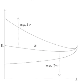
5) The relationship (10) leads to different position and shape of the optimal stopping boundaries b (see Figure 1). We divide it into three different regimes with µc is large, µc close to r and an intermediate case. We see when µc>r is relatively large, the boundary b is an increasing function of t and when µc close to r, the boundary b is a U-skewed shape. If we make µc move from ∞ to r, the optimal stopping boundary b will go up from 0 function gradually passing through the three shapes above with b T

( )

=K.

4. The Arbitrage-Free Price and the Rational Exercise

Boundary

In this section we will derive a closed form expression for the arbitrage-free price V in terms of the rational exercise boundary b (the early-exercise premium re-presentation).

We will make use of the following functions in Theorem 2 below:

( )

( )

( )

_{( )}

, c , e r T t r ,

F t x =Gµ t x − − − G t x (33)

(

)

( )

_{( ) (}

₎

0

, , , e r v t z c , , , d

[image:7.595.289.460.516.688.2]

J t x v z = − − −

∫

Hµ v y f v t x y− y (34)

DOI: 10.4236/jmf.2019.94038 754 Journal of Mathematical Finance for t∈

[

0,T

)

,x>0,v∈

( )

t T, and y>0, where functions Gr and _Gµc are given in (15) above, the function _Hµc is given in (21) and (25) above, and

(

, ,

)

y f v t x y− is the probability density function of xZv tr− from (14) above with µc replaced by r and T−t replaced by v−t

(

)

1 1

(

)

(

2

)

(

)

, , log 2

f v t x y y x r v t

y v tϕ v t σ

σ σ

 _{ }

− = _{ } − − − _

−  −  (35)

for y>0 where ϕ is defined as in (25) above. Note that since _Hµc

( )

_{v y}, <0

for all y∈

(

0,b v

( )

)

as b lies below h, then it is easy to verify that

( )

(

, , ,

)

0

J t x v b v > for all t∈

[

0,T

)

,x>0,v∈

( )

t T, . It is easy to see that

(

)

( ) 1 2

₍

₎

, , , e log

2

r T t z K

J t x T z r r T t

x T t

σ σ

− −   ∧   

− = Φ_  − −  − _

−    

  (36)

which is positive almost surely. It means that no matter what value z is, the buy-er should exbuy-ercise the option at the vbuy-ery closing time t=T . It follows what we

get in (26) that b T

( )

tends to be K.

Theorem 2 The arbitrage-free price of the British cash-or-nothing put option follows the early-exercise premium representation

( )

_{, e r T t}( ) _r

_{( )}

_, T

₍

_{, , ,}

_{( )}

₎

_d t

V t x = − − G t x +

∫

J t x v b v v (37)

for all

( )

t x, ∈

[ ]

0,T ×

(

0,∞

)

, where the first term is the arbitrage-free price of

the European put option and the second term is the early-exercise premium. The rational exercise boundary of the British put option can be characterised as the unique continuous solution b: 0,

[ ]

T →R+ to the nonlinear integral eq-uation

( )

(

,

)

T

(

,

( )

, ,

( )

)

d

t

F t b t =

∫

J t b t v b v v (38)

satisfying 0≤b t

( )

≤h t

( )

for all t∈

[ ]

0,T where h is defined by (26) above.

Proof. We will first derive (37) and (38). Then we will show the uniqueness of (38).

1) Let V: 0,

[ ]

T ×

(

0,∞ →

)

R and b: 0,

[ ]

T →R+ denote the unique solu-tion to the free-boundary problem (27)-(31), set

( )

[

) (

)

( )

{

, 0, 0, |

}

b

C = t x ∈ T × ∞ x>b t and

( )

[ ) (

)

( )

{

, 0, 0, |

}

b

D = t x ∈ T × ∞ x<b t , and let

( )

( )

2 2

( )

, , ,

2

XV t x rxV t xx x Vxx t x σ

= +

 for

( )

t x, ∈CbDb.

We summarize that V and b are continuous functions satisfying the following conditions:

• _{V is} 1,2

C on CbDb;

• _{b is of bounded variation;}

• P

(

Xt=c

)

=0 for all t∈

[ ]

0,T and c>0;

• Vt+XV−rV is locally bounded on CbDb;

•

(

,

( )

)

c

(

,

( )

)

x x

DOI: 10.4236/jmf.2019.94038 755 Journal of Mathematical Finance From these conditions we see that the local time-space formula is applicable to

( )

s y, →e−rsV t

(

+s xy,

)

with t∈

[

0,T

)

and x>0 given and fixed (see [11]). This leads to

(

)

( )

(

)(

)

(

(

)

)

(

) (

)

(

)

(

(

)

)

( )

0 0 e ,

, e , d

1

e , , d

2

rs

s

s _{rv b}

t X v v s

s _{rv b x}

x _v x _v v v

V t s xX

V t x V V rV t v xX I xX b t v v M

V t v xX+ V t v xX − I xX b t v X

− − − + = + + − + ≠ + + + + − + = +

∫

∫



 (39)

where Msb σ ₀se rvxX V tv x

(

v xX, v

)

dBv −

=

_∫

+ is a continuous local martingale for

[

0,

]

s∈ T−t and

( )

(

( )

)

0

b x b x

v

v s

X X

≤ ≤

=

  is the local time of

(

)

0

x

v _{v s}

X = xX _{≤ ≤}

on the curve b for s∈

[

0,T−t

]

. Furthermore, since V satisfies (27) on Cb and equals _Gµc on

b

D , and the smooth-fit condition holds at b, we see that (39)

implies

(

)

( )

₀

(

)(

)

(

(

)

)

e ,

, e , d

rs

s

s _{rv b}

t X v v s

V t s xX

V t x V V rV t v xX I xX b t v v M

−

−

+

= +

_∫

+_ − + < + + (40)

for s∈

[

0,T−t

]

and

( )

t x, ∈

[

0,T

) (

× 0,∞

)

.

2) Since b s

M is a continuous local martingale, there exists a sequence of

stopping times τn such that τn↑ ∞ as n↑ ∞ and the stopped process

n s

M ∧τ is a martingale. Replacing s by s∧τn in (40), we get

( )

(

)

( )

₀

(

)(

)

(

(

)

)

e ,

, e , d .

n n n n r s n s

s _{rv b}

t X v v s

V t s xX

V t x V V rV t v xX I xX b t v v M

τ τ τ τ τ − ∧ ∧ ∧ ₋ ∧ + ∧

= +

_∫

+_ − + < + + (41)

The martingale term vanishes when taking E on both sides. It follows

( )

(

)

( )

₀

(

)

(

(

)

)

E e ,

, E e , d

n n n _c r s n s s _rv v v

V t s xX

V t x H t v xX I xX b t v v

τ τ τ _µ τ − ∧ ∧ ∧ ₋  _{+ ∧}     

= + _ + < + _



∫



(42)

where _Hµc

( )

_{t x}, is well defined in (25). When taking _lim

n↑∞, it reduces to

(

)

( )

₀

(

)

(

(

)

)

E e ,

, E e c , d

rs

s

s _rv

v v

V t s xX

V t x Hµ t v xX I xX b t v v

−

−

 + 

 

 

= + _

_∫

+ < + _ (43)

3) Replacing s by T−t in (43), using that _{V T x}

( )

, =_Gµc

( ) (

_{T x}, =_{I x}≤_K

)

for x>0 and from the optimal sampling theorem, we get

( )

₍

₍

₎

₎

( )

(

)

(

(

)

)

( )

(

( )

)

0

e E

, e E , d

, , , , d .

c r T t

T t

T t _rv

v v

T

t

I xX K

V t x H t v xX I xX b t v v

V t x J t x v b v v

µ − − − − ₋ <  

= + _ + < + _

= −

∫

∫

(44)

Note that the left-hand side of (44) is e−r T t( −)Gr

( )

t x, and we will get the

ex-pression (37). It follows by (38) since _{V t b t}

(

,

( )

)

=_Gµc

(

_{t b t},

( )

)

for all

[ ]

0,

DOI: 10.4236/jmf.2019.94038 756 Journal of Mathematical Finance 4) We will show that the rational exercise boundary is the unique solution to (38) in the class of continuous functions t→b t

( )

on

[ ]

0,T satisfying

( )

( )

0≤b t ≤h t for all t∈

[ ]

0,T . To prove this, we assume a continuous

func-tion c: 0,

[ ]

T →R which solves (38) and satisfies 0≤c t

( )

≤h t

( )

for all

[ ]

0,

t∈ T . From (44), the function Uc: 0,

[ ]

T ×

(

0,∞ →

)

R is defined by

( )

( )

₍

₎

(

)

(

(

)

)

0

, e E ,

e E , d

c

c r T t

c

t t

T t _rv

v v

U t x G T xX

H t v xX I xX c t v v

µ µ − − − − ₋   = _{ }  

−

_∫

_ + < + _ (45)

for

( )

t x, ∈

[ ]

0,T ×

(

0,∞

)

. It is easy to know that if c solves (38) then

( )

(

,

)

c

(

,

( )

)

c

U t c t =Gµ t c t for all t∈

[ ]

0,T .

a) First we will show that _Uc

( )

_{t x}, =_Gµc

( )

_{t x}, for all

( )

[ ]

(

)

, 0, 0,

t x ∈ T × ∞

such that x≤c t

( )

. Take such

( )

t x, and the Markov property of X implies

(

)

₀

(

)

(

(

)

)

ers c , se rv c , d

s v v

U t s xX Hµ t v xX I xX c t v v

− _{+ −} − _{+ < +}

∫

(46)

is a continuous martingale under P for s∈

[

0,T−t

]

. Consider the stopping time

[

]

(

)

{

}

inf 0, |

c s T t xXx c t s

σ = ∈ − ≥ + (47)

under P. We see that

(

,

)

c

(

,

)

c c

c

c c

U t+σ xX_σ =Gµ t+σ xX_σ since

( )

(

,

)

c

(

,

( )

)

c

U t c t =Gµ t c t for all t∈

[ ]

0,T and _Uc

( )

_{T x}, =_Gµc

( )

_{T x}, for all

0

x> . Now we replace s by σc in (46) and take E on both sides, from the op-tional sampling theorem

( )

(

)

(

)

(

(

)

)

(

)

(

)

( )

0 0

, E e ,

E e , d

E e , E e , d

, c

c

c _c

c

c c c

c c r c c c rv v v r rv c v

U t x U t xX

H t v xX I xX c t v v

G t xX H t v xX v

G t x

σ

σ

σ _µ

σ

σ µ µ

σ µ σ σ − − − −   = _ + _  

− _ + < + _

      = _ + _− _ + _ =

∫

∫

(48)

where we use (22) in the last step.

b) Next, we will show that Uc

( )

t x, ≤V t x

( )

, for all

( )

t x, ∈

[ ]

0,T ×

(

0,∞

)

.

Then we consider the stopping time

[

]

(

)

{

}

inf 0, |

c s T t xXs c t s

τ = ∈ − ≤ + (49)

under P.

If x≤c t

( )

then τc =0 so that

( )

,

( )

,

c c

U t x =Gµ t x from a) above. On the

other hand, if x>c t

( )

then _Uc

(

_{t c t},

( )

)

=_Gµc

(

_{t c t},

( )

)

and

( )

, c

( )

,

c

U T x =Gµ T x for all x>0. From above analysis, we claim that

(

,

)

c

(

,

)

c c

c

c c

U t+τ xXτ =Gµ t+τ xXτ . Replacing s by τc in (46) and taking E on both sides, from the optional sampling theorem we get

( )

(

)

(

)

(

(

)

)

(

)

( )

0

, E e ,

E e , d

E e ,

, c c c _c c c c r c c c rv v v r c

U t x U t xX

H t v xX I xX c t v v

G t xX

V t x

τ τ τ _µ τ µ τ τ τ − − −   = _ + _  

− _ + < + _

 

= _ + _

≤

DOI: 10.4236/jmf.2019.94038 757 Journal of Mathematical Finance where

( )

,

(

)

0

, sup E e r c , .

t x T t

V t x τGµ t xXτ

τ τ

− ≤ ≤ −

 

= _ + _ (51)

Therefore, Uc

( )

t x, ≤V t x

( )

, as claimed.

c) Next, we are going to show that b t

( ) ( )

≤c t for all t∈

[ ]

0,T . We will prove

in reverse. Suppose that there exists t∈

[ ]

0,T such that c t

( ) ( )

<b t . Take any

( )

x≤c t and consider the stopping time

[

]

(

)

{

}

inf 0, |

b s T t xXs b t s

σ = ∈ − ≥ + ₍₅₂₎

under P. Replacing s with σb in (40), taking E on both sides and applying the optional sampling theorem we get

(

)

( )

₀

(

)

E e b , , E be c , d .

b

r rv

b v

V t xX V t x σ H t v xX v

σ µ

σ

σ

−  − 

 ₊ _{= +  + }

  _

∫

_ (53)

Repeating the above process in (46), we find

(

)

( )

₀

(

)

(

(

)

)

E e ,

, E e , d .

b b b _c r c b c rv v v

U t xX

U t x H t v xX I xX c t v v

σ σ σ _µ σ − −  +     

= + _ + < + _



∫



(54)

We see _Uc

( )

_{t x}, =_Gµc

( )

_{t x}, =_{V t x}

( )

, since _x≤_{c t}

( )

and by b) we know

(

,

) (

,

)

b b

c

b b

U t+σ xX_σ ≤V t+σ xX_σ , then (53) and (54) imply that

(

)

(

(

)

)

0

E berv c , d 0.

v v

H t v xX I xX c t v v

σ _{− µ}

 _{+ ≥ +} _≥

 



∫

 (55)

On the other hand, the fact that b lies below h forces (55) to be strictly nega-tive and provides a contradiction. Therefore, c t

( ) ( )

≥b t as claimed.

d) Next, we will show that b t

( ) ( )

=c t for all t∈

[ ]

0,T . We first assume that

there exists t∈

[ ]

0,T such that c t

( ) ( )

>b t . Take any x∈

(

c t b t

( ) ( )

,

)

and

consider the stopping time

[

]

(

)

{

}

inf 0, |

b s T t xXs b t s

τ = ∈ − ≤ + (56)

under P. Replacing s with τb in (40) and (46), taking E on both sides and ap-plying the optional sampling theorem we get

(

)

( )

E e b , ,

b r

b

V t xX V t x

τ

τ τ −

 + =

  (57)

(

)

(

)

(

(

)

)

0

E e ,

( , ) E e , d .

b b b _c r c b c rv v v

U t xX

U t x H t v xX I xX c t v v

τ τ τ _µ τ − −  +     

= + _ + < + _



∫



(58)

We see that

(

,

)

c

(

,

) (

,

)

b b b

c

b b b

U t+τ xX_τ =Gµ t+τ xX_τ =V t+τ xX_τ by a) and c)

above since b≤c. Furthermore, by b) we know Uc ≤V so (57) and (58) leads

to

(

)

(

(

)

)

0

E be rv c , d 0.

v v

H t v xX I xX c t v v

τ _{− µ}

 _{+ < +} _≥

 



∫

 (59)

DOI: 10.4236/jmf.2019.94038 758 Journal of Mathematical Finance

5. Financial Analysis of the British Cash-or-Nothing Put

Option

In this section, we focus on the practical features of the British cash-or-nothing put option. We compare it with the American put option that is universally traded. We address the problem as to what the return would be if the price of the underlying asset enters the given region at a given time.

1) As shown in Figure 1, the rational exercise strategy of the British cash-or-nothing put option varies with different contract drift µc. Recall that

c r

µ > _{since if the opposite condition occurs, the option holder is overprotected} by exercising the option at once. Furthermore, he can also avoid any discounting of the payoff. We also noted above that b T

( )

=K. In particular, if µc =r the boundary tends to be infinity backwards in time from T, which means it is op-timal to stop immediately at the very beginning of time. The interest rate r stands for a infinite boundary and any µc >r represents a non-trivial rational exercise boundary. On the other hand, when µc↑ ∞ the boundary decreases sharply to 0 backwards from b T

( )

=K. The option buyer should hold the

op-tion till maturity and it is not opop-tional to exercise the opop-tion before time T. In this case the ∞ represents an infinite tolerance of the true drift and reduces the British cash-or-nothing put option to European cash-or-nothing put option. All above, the contract drift µc should not be set too close to r or too large since the former case leads to overprotection and the latter reduces it to a European style option.

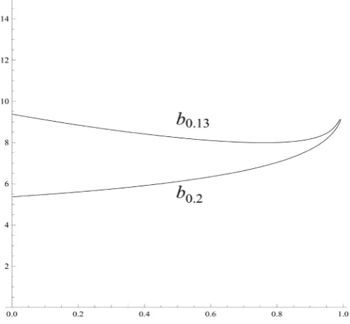
2) We have mentioned above that the “overprotection” in this paper mainly refers to the initial stock price is below K which leads to the option holder is overprotected as the highest boundary in Figure 1 shown. Although bigger than the interest rate r, the contract drift is favourable enough to exercise the option immediately. Figure 2 compares the rational boundaries with different fixed pa-rameters. In addition to this, the values of the boundary have a strong relation-ship with the volatility σ . With larger volatility, the option buyer has a greater tolerance of the drift. This is due to the “drown-out” effect of the higher volatili-ty i.e. the option holder tends to believe that the high volatility can drown out the loss of the drift. In this case, the boundary b is likely to be more U-skewed with larger b

( )

0 . Therefore, the contract drift µc should be set further away from the interest rate r with larger volatility. On the other hand, Figure 2 also illustrates the fact that if the contract drift µc is set closer to the interest rate r, the British cash-or-nothing put option will be more expensive since the over-protection feature is stronger.

3) Assume that the initial stock price is 11. The price of the European cash-or-nothing put option is 0.3498 with K=10, T =1, r=0.1 and

0.4

σ = _{. The price of the American cash-or-nothing put option is 0.7885 and}

the price of the British cash-or-nothing put option is 0.3597 with µ_c =0.13 and

0.3536 with µ_c =0.2. We get that the closer the contract drift gets to r, the

[image:13.595.248.500.75.308.2]

DOI: 10.4236/jmf.2019.94038 759 Journal of Mathematical Finance

Figure 2. A computer drawing showing the rational exercise boundary of the British cash-or-nothing put option with K=10, T=1,

0.1

r= , σ =0.4 when µc=0.13 and µc=0.20.

European option and the American option. If the contract drift µc is too close to r, the protection feature works and makes the price of the British option ex-tremely close to the American option. On the other hand, if µc ↑ ∞ the British cash-or-nothing put option will be reduced to the European cash-or-nothing put option. Therefore, we conclude that the price of the British cash-or-nothing put option lies above the European option and below the American option.

4) Table 1 illustrates the power of the protection feature in practice. For in-stance, if the stock price is 11 halfway to maturity then the option holder can ex-ercise to a payoff with a reimbursement of 66% - 74% of the initial investment. However, in the case of the American cash-or-nothing put option, the holder is out-of-the-money and would receive zero payoff. We see that the size of the reimbursement also varies with the contract drift as analyzed in the former pa-ragraph. When the contract drift gets closer to r, the option holder gets more protection as well as greater reimbursement.

[image:14.595.209.540.216.421.2]

DOI: 10.4236/jmf.2019.94038 760 Journal of Mathematical Finance put option. However, in the real market the option holder’s ability to sell the op-tion is affected by many exogenous factors such as the fricop-tion costs, taxes the liquidity of the market and so on. Therefore, from this point of view it makes the British style option more attractive since the protection feature to the British op-tion is intrinsic and endogenous.

Table 1. Returns observed upon exercising the British cash-or-nothing put option at and above the strike price K. The returns are calculated by _{R t x}

( )

, =_Gµc

( ) (

_{t x V}, 0,_K

)

. The

parameter set is same as in Figure 2 i.e. K=10, T=1, r=0.1, σ =0.4 and the

initial stock price is 10.

Time(months) 0 2 4 6 8 10 12

Exercise at 10 with µ =c 0.13 100% 101% 102% 103% 105% 106% 222% Exercise at 10 with µ =c 0.20 87% 89% 92% 94% 98% 102% 227% Exercise at 11 with µ =c 0.13 80% 79% 77% 74% 70% 58% 0% Exercise at 11 with µ =c 0.20 67% 67% 67% 66% 63% 55% 0% Exercise at 12 with µ =c 0.13 62% 60% 57% 51% 43% 27% 0% Exercise at 12 with µ =c 0.20 51% 50% 48% 44% 38% 24% 0% Exercise at 13 with µ =c 0.13 48% 45% 41% 34% 25% 11% 0% Exercise at 13 with µ =c 0.20 39% 36% 33% 29% 22% 10% 0% Exercise at 14 with µ =c 0.13 37% 33% 29% 22% 14% 4% 0% Exercise at 14 with µ =c 0.20 29% 26% 23% 18% 12% 3% 0% Exercise at 15 with µ =c 0.13 28% 25% 20% 14% 7% 1% 0% Exercise at 15 with µ =c 0.20 21% 19% 16% 11% 6% 1% 0%

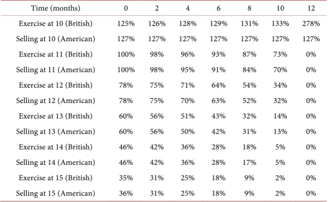
Table 2. Returns observed upon exercising the British cash-or-nothing put option (with

0.13 c

µ = ) at and below the strike price K compared with the American cash-or-nothing put option in the same contingency. The returns are calculated by

( )

, c

( ) (

, 0,11

)

R t x =Gµ t x V and R_A

( )

t x, =G_A

( )

t x V, _A

(

0,11

)

respectively. The

parameter set is same as in Figure 2 i.e. K=10, T=1, r=0.1, σ =0.4 and the

initial stock price is 11.

Time (months) 0 2 4 6 8 10 12

[image:14.595.208.539.516.728.2]

[image:15.595.209.540.156.360.2]

DOI: 10.4236/jmf.2019.94038 761 Journal of Mathematical Finance

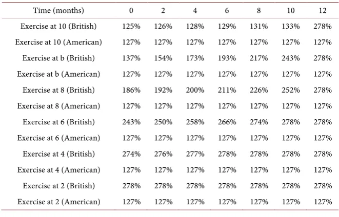
Table 3. Returns observed upon exercising the British cash-or-nothing put option (with

0.13 c

µ = _{) at and above K compared with selling the American cash-or-nothing put}

option in the same contingency. The returns are calculated by

( )

, c

( ) (

, 0,11

)

R t x =Gµ t x V and R_A

( )

t x, =V_A

( )

t x V, _A

(

0,11

)

respectively. The

parameter set is same as in Figure 2 i.e. K=10, T=1, r=0.1, σ =0.4 and the

initial stock price is 11.

Time (months) 0 2 4 6 8 10 12

Exercise at 10 (British) 125% 126% 128% 129% 131% 133% 278% Selling at 10 (American) 127% 127% 127% 127% 127% 127% 127% Exercise at 11 (British) 100% 98% 96% 93% 87% 73% 0% Selling at 11 (American) 100% 98% 95% 91% 84% 70% 0% Exercise at 12 (British) 78% 75% 71% 64% 54% 34% 0% Selling at 12 (American) 78% 75% 70% 63% 52% 32% 0% Exercise at 13 (British) 60% 56% 51% 43% 32% 14% 0% Selling at 13 (American) 60% 56% 50% 42% 31% 13% 0% Exercise at 14 (British) 46% 42% 36% 28% 18% 5% 0% Selling at 14 (American) 46% 42% 36% 28% 17% 5% 0% Exercise at 15 (British) 35% 31% 25% 18% 9% 2% 0% Selling at 15 (American) 36% 31% 25% 18% 9% 2% 0%

6. Other British Binary Options

We remarked above that the British binary option analyzed in this paper plays a cononical role among all other possibilities. The aim of this section is to provide a brief review of other British binary options as discussed in Section 1. Extending Definition 1 of Section 3 in an obvious manner we obtain the following classifi-cation of British binary options (according to their payoffs):

• _{The British cash-or-nothing call option:}

(

)

E c |

T t

I X K

µ _{ > }

  (60)

• _{The British asset-or-nothing call option:}

(

)

E c |

T T t

X I X K

µ _{ > }

  (61)

• _{The British asset-or-nothing put option:}

(

)

E c |

T T t

X I X K

µ _{ < }

  (62)

with µc is a contract drift.

Acknowledgements

The author is grateful to Professor Goran Peskir, Yerkin Kitapbayev and Shi Qiu for the informative discussions.

Conflicts of Interest

DOI: 10.4236/jmf.2019.94038 762 Journal of Mathematical Finance

References

[1] Geske, R. (1979) The Valuation of Compound Options. JournalofFinancial Eco-nomics, 7, 63-81. https://doi.org/10.1016/0304-405X(79)90022-9

[2] Gukhal, C.R. (2004) The Compound Option Approach to American Options on Jump-Diffusions. JournalofEconomicDynamicsandControl, 28, 2055-2074.

https://doi.org/10.1016/j.jedc.2003.06.002

[3] Black, F. and Scholes, M. (1973) The Pricing of Options and Corporate Liabilities.

TheJournalofPoliticalEconomy, 81, 637-654. https://doi.org/10.1086/260062

[4] Peskir, G. and Samee, F. (2011) The British Put Option. Applied Mathematical Finance, 18, 537-563. https://doi.org/10.1080/1350486X.2011.591167

[5] Peskir, G. and Samee, F. (2013) The British Call Option. QuantitativeFinance, 13, 95-109. https://doi.org/10.1080/14697688.2012.696676

[6] Merton, R.C. (1973) Theory of Rational Option Pricing. TheBellJournalof Eco-nomicsandManagementScience, 4, 141-183. https://doi.org/10.2307/3003143

[7] Glover, K., Peskir, G. and Samee, F. (2010) The British Asian Option. Sequential Analysis, 29, 311-327. https://doi.org/10.1080/07474946.2010.487439

[8] Glover, K., Peskir, G. and Samee, F. (2011) The British Russian Option. Stochastics:

AnInternationalJournalofProbabilityandStochasticProcesses, 83, 315-332.

https://doi.org/10.1080/17442501003690192

[9] Shiryaev, A.N. and Kruzhilin, N. (1999) Essentials of Stochastic Finance: Facts, Models, Theory. World Scientific, Singapore.

https://doi.org/10.1142/9789812385192

[10] Al-Fagih, L. (2015) The British Knock-In Put Option. International Journal of TheoreticalandAppliedFinance, 4, 355-359.

[11] Al-Fagih, L. (2015) The British Knock-Out Put Option. International Journal of TheoreticalandAppliedFinance, 18, Article ID: 1550008.

https://doi.org/10.1142/S0219024915500089

[12] Kitapbayev, Y. (2015) The British Lookback Option with Fixed Strike. Applied Ma-thematicalFinance, 22, 238-260. https://doi.org/10.1080/1350486X.2015.1019156

[13] Peskir, G. and Shiryaev, A. (2006) Optimal Stopping and Free-Boundary Problems. Birkhäuser, Basel.

[14] Peskir, G. (2005) A Change-of-Variable Formula with Local Time on Curves. Jour-nalofTheoreticalProbability, 18, 499-535.