Michael B. Morrissey 2
August 28, 2014 3
School of Biology, University of St Andrews 4
5
contact
email: [email protected] phone: +44 (0) 1334 463738
fax: +44 (0) 1334 463366
post: Dyers Brae House
School of Biology, University of St Andrews St Andrews, Fife, UK, KY16 9TH
Keywords: natural selection, selection gradients, colinearity, tables of statistics, regularised 6
regression, projection-pursuit regression, informative priors 7
Abstract
8
1. Regression is an important method for characterising the form of natural selection from 9
individual-based data. Many kinds of regression analysis exist, but few are regularly em-10
ployed in studies of natural selection. I provide an overview of some of the main underused 11
types of regression analysis by applying them all to test analyses of viability selection for 12
lamb traits in Soay sheep (Ovis aries). This exercise highlights known problems with
exist-13
ing methods, uncovers some new ones, and also reveals ways to harness underused methods 14
to get around these problems. 15
2. I first estimate selection gradients using generalised linear models, combined with recently-16
published methods for obtaining quantitatively interpretable selection gradient estimates 17
from arbitrary regression models of trait-fitness relationships. I then also apply generalised 18
ridge regression, the lasso, and projection-pursuit regression, in each case also deriving 19
selection gradients. I compare inferences of non-linear selection by diagonalisation of the 20
matrix and by projection-pursuit regression. 21
3. Selection gradient estimates generally correspond across di↵erent regression methods.
Al-22
though there is little evidence for non-linear selection in the test datasets, very problematic 23
aspects of the behaviour of analysis based on diagonalisation of the are apparent. In
addi-24
tion to better-known problems, (i) the direction and magnitude of estimated major axes of 25
quadratic selection are biased toward directions of phenotype that have little variance, and 26
(ii) the magnitudes of selection of major axes of variance-standardised are not themselves
27
interpretable in any standardised way. 28
4. While all regression-based methods for analysis of selection have useful properties, projection-29
pursuit regression seems to stand out. This method can: (i) provide both dimensionality-30
reduction, (ii) be the basis for inference of quantitatively interpretable selection gradients, 31
and (iii) by characterising major axes of selection, rather than of linear or quadratic selec-32
1
Introduction
34
Understanding multivariate microevolutionary parameters is currently one of the key challenges 35
of evolutionary quantitative genetics (Blows, 2007; Philips & Arnold, 1989; Walsh & Blows, 36
2009). It is now well established that univariate and bivariate views of the genetics and selec-37
tion of ecologically-important traits can, and perhaps even generally will, fail to reveal critical 38
aspects of microevolutionary processes, including selected axes of phenotype and genetic con-39
straints (Dickerson, 1955; Ro↵ & Fairbairn, 2007). Furthermore, microevolutionary parameters
40
of natural populations are likely to vary with many aspects of population structure, including 41
age and sex (Lande & Arnold, 1983; Poissant et al., 2008), space (Siepielski et al., 2013), time 42
(Bell, 2010; Morrissey & Hadfield, 2012; Siepielski et al., 2009), and environmental conditions 43
generally (Carlson & Quinn, 2007; Grant & Grant, 2002; MacColl, 2011). Consequently, char-44
acterisation of key aspects of the evolutionary process is generally very challenging, not only in 45
the ecological insight required to conceive data collection strategies and conduct analyses, but 46
also in that collection of required quantities of relevant data in realistic conditions and under 47
any particular regime of population structure is often very difficult. Here, I consider methods for 48
multivariate selection analysis with special focus on the biological interpretability of inferences 49
about multivariate selection from limited data. I consider viability selection of skeletal size, 50
mass, horn length, and burden of an ectoparasite in male and female Soay sheep lambs under 51
two di↵erent population dynamic regimes.
52
The best known pitfall of interpreting tables of statistical results is the problem of multiple 53
testing and false positives (Rice, 1989). Less appreciated complexities pertain to statistical 54
estimates themselves. Biological interpretation of statistical inferences about natural selection 55
generally involves consideration of tables of selection coefficients. Tables of estimated selection 56
coefficients will generally have very undesirable properties. Many of the aspects of selection in 57
which we may be primarily interested are not represented by individual selection coefficients,
58
but rather are obtained by applying mathematical procedures to tables of estimated selection 59
coefficients (gradients, typically). Even when applied to a table of selection coefficients that 60
are obtained by an unbiased method, few properties of tables of selection coefficients will have
desirable statistical properties, and in general, “doing statistics on statistics” can easily generate 62
complex statistical artefacts that can appear to represent meaningful and interesting biological 63
results. 64
A simple illustration of potential biases in interpreting tables of evolutionary quantitative 65
genetic parameters arises from the geometric interpretation of the multivariate selection gradient. 66
The length of the gradient, or its vector norm, denoted || ||, represents an important aspect
67
of the total strength of multivariate directional selection. In multivariate studies, geometric 68
properties such as|| ||are often integral to the best theory that we can apply to understanding
69
how selection and genetics interact to generate evolutionary trajectories (Hansen & Houle, 2008; 70
Walsh & Blows, 2009). However, the length of an estimated selection gradient vector – even 71
one composed of individually unbiased component selection gradient estimates such as those 72
generated by multiple regression analysis (Lande & Arnold, 1983; Morrissey & Sakrejda, 2013) 73
– is biased in a potentially biologically misleading way. 74
A simplified model is instructive. Consider a vector of k selection gradients, with equal
75
absolute values of b, i.e., the true value of selection for each trait (for whatever scaling of
76
phenotype has been deemed appropriate for the study) is equal. Consider that this true selection 77
gradient is estimated with error. Assume that each estimated selection gradient ˆi is drawn
78
from a normal distribution according to ˆi ⇠N(bi, s2), so, each estimated gradient is unbiased,
79
sampling errors are independent, and standard errors, s, are equal across estimates. The true
80
norm of ispkb2. The expected value of the sum of squared estimated elements of isk(b2+s2),
81
as opposed to the sum of the true squared elements, which is kb2. An exact expression for the
82
expected value of the norm of ˆ is not easily obtained. However, since px is a monotonic
83
function of x, it follows from k(b2 +s2) kb2 that E[||ˆ||] must be greater than || ||, i.e.,
84
upwardly biased, whenever s >0. 85
A first order approximation for E[||ˆ||] is thus pk(b2+s2), and this allows us to start to
86
get a handle on the nature of this upward bias. Bias is normally expressed as the di↵erence
87
between the expected value of an estimator, e.g., E[ˆx], and the true value of the estimator’s
88
target estimand, x. Here, where both the true and estimated values of the length of a vector
89
(which will have a value of 1 in the absence of bias) in terms of the proportional sampling error, 91
p= sb. Substituting pb fors in the expressions above and simplifying gives 92
E[||ˆ||]
|| || ⇡
p
1 +p2.
This again indicates that estimates of the length of , given individually unbiased component
93
elements of ˆ , will be upwardly biased1. Furthermore, this expression illustrates that the problem
94
is severe. Since standard errors of selection gradients are generally as large as most selection 95
gradients (sop⇡1; remembering that the distribution of selection gradients in the literature also 96
provides an upwardly biased impression of the average magnitude of selection; Hereford et al.
97
2004), upward bias in the estimated strength of multivariate directional selection on the order of 98
40% should be expected. Also, the assumptions of the instructive example should not hinder the 99
generality of its interpretation. The basic principle will hold for arbitrary distributions of true 100
values of selection gradients. Furthermore, sampling covariances among elements of ˆ , as arise 101
from phenotypic covariances, will cause larger biases than the simple calculation suggests. This 102
is the principle of variance inflation under multicolinearity, which has recently been reviewed by 103
Dormannet al. (2013) in the context of ecological statistics.
104
The goal of this study is to explore a variety of approaches to selection analysis, in order to 105
determine what methods hold the most promise for making robust inferences of di↵erent aspects
106
of multivariate selection. I apply a range of regression methods to analyses of multivariate 107
selection of Soay sheep lamb traits, including generalised linear models, regularised generalised 108
regression models, and projection-pursuit regression. I use a recently-described approach for 109
obtaining selection gradient estimates from general fitness functions (Morrissey & Sakrejda, 110
2013) to obtain quantitative inferences of selection gradients from each of these analyses. I also 111
explore the properties of estimated major axes of quadratic selection, and of selection analysis 112
of principle components of the multivariate phenotype. These methods all provide tables of 113
selection gradients that may di↵er in bias, and other aspects of informativeness, with respect to 114
1This approximation for the proportional bias is itself somewhat upwardly biased. If selection gradients can be scaled such that
their standard errors are equal to one (as a hypothetical instructive situation), the expected norm of the estimated selection gradient vector is given by the expectation of a chi distribution. This does not lead to a simple informative expression, but numerical analysis shows that the approximation E|| ||[||ˆ||] ⇡p1 +p2 upwardly estimates the bias by about 10% forkandp⇡0.7, and is otherwise a
di↵erent aspects of multivariate selection. 115
2
Methods and Results
116
2.1 Example study system and data
117
Soay sheep on Hirta, St Kilda, in the Outer Hebrides, have been monitored in an individual-based 118
study since 1984 (Clutton-Brock & Pemberton, 2004). The portion of the phenotypic data used 119
here are collected each August, when a large portion of the Soay sheep resident in the Village 120
Bay study area are captured. I analyse body mass (kg), hind leg length (mm), horn length 121
(mm), and number of keds (Melophagus ovinus), an ectoparasite, of lambs measured in August.
122
Aspects of size have previously been shown to be related to survival (e.g., Clutton-Brocket al.
123
1992; Milneret al.1999), and to have complex phenotypic and genetic covariances with lifetime
124
fitness (Morrissey et al., 2012a). Horn size is also closely related to aspects of both survival and 125
reproduction (Coltmanet al., 1999; Johnstonet al., 2013; Robinsonet al., 2006). Although keds 126
cause some skin irritation (Wilson et al., 2004) their presence or prevalence has not previously
127
been related to fitness, and this parasite does not appear to impact negatively on other aspects 128
of sheep performance. I focus on traits in lambs, and furthermore restrict the dataset to those 129
individuals with the normal horn morph (Clutton-Brock & Pemberton, 2004). 130
The month, and usually day, of death is known for nearly all individuals, allowing us to 131
determine viability from the time of measurement in August through to one year of age, defined 132
operationally as 1st April in the year following birth. The Soay sheep population experiences a
133
wide range of over-winter survival rates, with pronounced crashes in some years (Clutton-Brock & 134
Pemberton, 2004). For all selection analyses, I therefore divide the dataset into four subsets, for 135
male and female lambs in crash and non-crash years. Cohorts born in springs prior to overwinter 136
crashes are: 1988, 1991, 1994, 1997, 2004 and 2011. Sample sizes and mean survival rates are: 137
males in non-crash years: n= 633, W¯ = 0.687, females in non-crash years: n = 213, W¯ = 0.803,
138
males in crash years: n = 281, W¯ = 0.359, and females in crash years: n = 117, W¯ = 0.470.
139
Sample size is smaller for females because the expression of the horn polymorphism is sex-specific, 140
and correlations among traits in each sex and environmental condition are given in table 1. All 142
traits, i.e., mass, leg length, horn length, and log ked number, were standardised to unit variance 143
within each of the four datasets. 144
2.2 General strategy for selection gradient estimation 145
Analyses in sections 2.3 - 2.7 all use a common framework for selection gradient estimation. 146
In each case, the relationship between multivariate phenotype and expected individual fitness, 147
E[Wi] = f(zi), is first determined using a generalised regression model. Subsequently,
pop-148
ulation mean fitness, given the sample of phenotypes z and the function f(z) is obtained by
149 ¯
W = n1 Pni f(zi). The first and second partial derivatives of population mean fitness with
re-150
spect to population mean phenotype are then calculated by numerical methods. When scaled 151
by dividing by population mean fitness, these derivatives provide estimates of directional and 152
quadratic/correlational selection gradients, i.e., i = Wz¯¯iW¯ 1, and i,j =
2W¯ ¯ zi ¯zj
¯
W 1, respectively.
153
This method is described in detail in Morrissey & Sakrejda (2013). Where appropriate, stan-154
dard errors were calculated and statistical hypothesis tests were applied using the parametric 155
bootstrap method also described in Morrissey & Sakrejda (2013). All traits were standardised 156
to unit variance. 157
The Morrissey & Sakrejda (2013) method for obtaining selection gradients estimates from 158
arbitrary inferences of E[Wi] = f(zi), directly calculates the partial derivatives of population
159
mean fitness with respect to population mean phenotype, scaled to the relative fitness. These 160
quantities are returned regardless of the distribution of phenotype. For example, if the distri-161
bution of one or more traits is skewed, the estimates of and will still reflect the first and
162
second partial derivatives of mean relative fitness with respect to phenotype. This definition of 163
relates to evolutionary change via z¯= G under the assumption that breeding values are
164
multivariate normal (see proof in appendix). In contrast, the estimates of and provided
165
by the familiar regression analysis described by equation 16 in Lande & Arnold (1983), will not 166
predict evolutionary change when the phenotype is not multivariate normal, even if breeding 167
values are MVN. 168
The shape off(zi), as obtained by generalised regression analysis, will be determined in part
by the link function. Iff(zi) is a linear function on the linear predictor scale, i.e., takes the form of
170
E[Wi] =link 1(µ+Pkjbjzi,j), then the curvature will be entirely determined by the shape of the
171
link function. Estimates of obtained from such a model of the fitness function will generally
172
provide robust inference of directional selection, but estimates of should not generally be
173
interpreted biologically. When quadratic, or otherwise curved (e.g., spline) generalised regression 174
models are used forf(zi), the link function will generally have very little e↵ect on estimates of
175
either or . For example, models of binary outcomes (e.g., survival) could equally be fitted
176
using logit or probit link functions. For any given dataset, the parameters of f(zi) will di↵er
177
between models using the logit and probit link functions, but the shape off(zi) on the expected
178
fitness scale, and therefore estimates of and , will typically di↵er trivially. 179
All analyses in the present work consider relatively simple distributions of fitness. In particu-180
lar, all analyses and empirical examples involve a binary (survival) fitness response. The method-181
ological focus is thus on aspects of inferring selection of the multivariate phenotype. These issues 182
should be seen as complimentary to other ongoing avenues for methodological development of 183
methods for the analysis of natural selection. The work here is hopefully complimentary to, 184
for example, methods for using information about the life cycle to construct sensible models of 185
variation in fitness (Geyer et al., 2007; Shaw & Geyer, 2010), e↵orts to characterise selection in 186
a demographic context (Engen & Saether, 2014; Engenet al., 2012; Morrisseyet al., 2012b), and 187
application of theory to disentangle purely correlative from direct and indirect e↵ects of traits 188
on fitness (Morrissey, 2014). 189
2.3 Selection di↵erentials and multiple regression-based estimation of selection gra-190
dients 191
I obtained variance-standardised directional selection di↵erentialsS for each trait by calculating 192
the di↵erence between mean phenotype weighted by fitness and mean phenotype before selection.
193
I obtained quadratic selection di↵erentials as C = P+SST, where P is a matrix of trait
194
variances and covariances, weighted by relative fitness, minus the variance and covariances before 195
selection, andSis the vector of directional selection di↵erentials. I obtained standard errors and 196
I obtained standardised directional and quadratic selection gradients by first fitting gener-198
alised linear models (glm) with a binomial responses, using theR package mgcv (Wood, 2006),
199
and (linear predictor scale) linear, quadratic, and interaction e↵ects for all traits and trait combi-200
nations, for each of the four datasets. I then obtained the selection gradient estimates from these 201
fitted models (see section 2.2), as implemented in the R package gsg (Morrissey & Sakrejda,
202
2013), with standard errors and p-values, using a parametric bootstrap. 203
Survival covaries positively with mass and leg length in both sexes and in both environmental 204
conditions (table 2a). In crash years only, but in both males and females, survival covaries 205
positively with horn size as well. No consistent patterns occur in changes in variances and 206
covariances due to selection, over and above those necessarily associated with changes in the mean 207
(Endler, 1986; Lande & Arnold, 1983), with the exceptions of some marginally non-significant 208
values, and one nominally significant value (i.e., without accounting for multiple tests) for the 209
change in the covariance of horn length and ked number. 210
Selection gradients revealed that covariance of survival with mass and leg length is primarily 211
directly attributable to variation in mass in non-crash years (table 2b). Also in non-crash 212
years, horn length has negative direct e↵ects on survival, again in both sexes, i.e., the slightly 213
positive and non-significant covariances of horn length and survival arise via opposite e↵ects of 214
correlated selection of mass, and direct selection of horn length. Inference of the direct causal 215
structure of selection in crash years appeared to be hindered in part by smaller sample sizes 216
for crash years, compared with the relatively high degree of correlation of phenotypic traits 217
(which happened across conditions; table 1). Importantly, this should not be taken as a lack of 218
statistically significant selection: the covariances of traits and fitness (table 2a), arise somehow, 219
and multiple regression analysis can only attribute this covariance to the traits that are included 220
in the analysis. Thus there is significant selection, but there is also a statistical failure to 221
robustly partition total selection into direct e↵ects among the available predictor variables. This 222
alone is an important property of a table of multiple regression coefficients, and potentially an 223
interpretive trap (see also discussion in Mitchell-Olds & Shaw 1987); non-significance of each 224
gradient in isolation (table 2b) does not correspond to non-significance of total selection (table 225
2.4 Major axes of the quadratic approximation of the fitness surface 227
I further investigated multivariate quadratic selection following methods discussed and promoted 228
by Philips & Arnold (1989) and by Blows (2007). To characterise the major orthogonal axes of 229
quadratic selection, I performed canonical rotations of each matrix of estimated quadratic and 230
correlational selection gradients 231
=M⇤MT (1)
where M is a matrix of orthogonal eigenvectors, and ⇤ is a diagonal matrix containing the
232
associated eigenvalues. Values in ⇤ are interpreted as the quadratic selection gradients of the
233
new independent axes of the quadratic component of the relative fitness surface. 234
I constructed null distributions of the magnitudes of the eigenvalues of the rotated matrices
235
using an algorithm very similar to that suggested by Reynoldset al.(2010). I first generated 1000 236
datasets with the original phenotypic data (separately for each combination of sex and crash vs. 237
non-crash conditions) and permuted values of fitness. I then re-fitted the multivariate quadratic 238
logistic regression model, and for each logistic model fitted to the permuted fitness data, I re-239
calculated the associated selection gradients, as above. From each set of selection gradients for 240
each permuted dataset, I rotated the matrix and recorded the eigenvalues (i.e., the quadratic
241
selection gradients of the diagonalised estimated matrix), ordered by their absolute values.
242
Statistical hypotheses tests associated with the comparison of observed values to permuted values 243
are given in table 3. 244
Some authors have reported statistical hypothesis tests of selection along axes with smaller 245
eigenvalues. While there is potentially some value in considering statistical hypothesis tests of 246
minor axes, when larger axes are non-significant, it is not clear that any interpretive gain could 247
outweigh the dangers of multiple testing. In the present analyses, across 16 tests of four axes of 248
quadratic selection, in each of both sexes and both crash and non-crash years, no permutation-249
based tests of any axis were statistically significant at a marginal value of 0.05 (table 1). 250
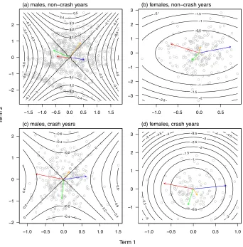
The major axis of the diagonalised matrix in both sexes and in both environments involved
251
loadings of mass and leg length in opposite directions (table 1). In other words, the main axis of 252
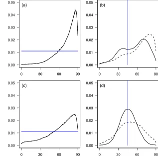
is probably an artefact of the fact that selection is most difficult to characterise in this direction, 254
and therefore sampling error will produce the largest errors in the direction of phenotype with 255
the least variance. A second interpretive difficulty is apparent in figure 1. Even though the
256
analysis is conducted on unit variance-standardised values of phenotype, the major axes of 257
cannot be interpreted with the benefits that come from variance standardisation. Despite the 258
fact that the first axes represent much greater absolute curvature than the second axes in each 259
case (table 3), the amount of variation in fitness associated with the first two axes - over the 260
distribution of phenotype in those directions - is very similar in two cases (figure 1a,c), and in 261
two cases the variance in fitness associated with the second estimated axis is clearly greater that 262
that associated with the first (figure 1b,d). 263
2.5 Regularised regression-based selection gradient estimates 264
Elastic net regularisation (Zou & Hastie, 2005) is a general form of biased regression estimation 265
that includes ridge regression (Tikhonov & Arsenin, 1977) and least absolute shrinkage and 266
selection operator (“the lasso”; Tibshirani 1996) as special cases. Where least squares regression 267
obtains estimated regression coefficients b by minimising ||y Xb||2, the elastic net minimizes
268
(||y Xb||2+↵||b||2+ (1 ↵)||b||). When ↵ = 1, the analysis is a ridge regression, and when
269
↵= 0, the analysis is the lasso. 270
Both ridge regression and the lasso thus minimise penalised sums of squares, with the goal 271
of maximising predictive ability, rather than fit to the sample data. In practice, ridge regression 272
reduces the overall magnitude of regression coefficients, relative to least-squares regression, and in 273
particular, gives more plausible values for regression coefficients associated with highly correlated 274
predictor variables. The lasso also produces shrunken values, but will generally shrink di↵erent
275
coefficients to a much greater extent, in particular, potentially assigning zero values to coefficients 276
associated with variables that have no probable predictive ability. Ridge regression and the lasso 277
therefore have properties that may be desirable overall, and that can be particularly desirable 278
when predictors are highly correlated, as is often the case in selection analysis. 279
I used generalised elastic net (with ridge regression and the lasso, and a combination of 280
the two with ↵ = 0.5) regression to estimate selection gradients, as above, by first estimating
fitness functions, and then obtaining selection gradient estimates from those functions. I used 282
the function cv.glmnet() in the R package glmnet (Friedman et al., 2008) to fit the ridge
283
regression, lasso and elastic net regressions (↵ = 0.5) with binomial responses by generalised
284
cross-validation, and used those estimated regression coefficients based on the penalty parameter 285
that minimised the cross-validation score. All estimated selection gradients derived from these 286
models of the fitness function are given in table 4. 287
In non-crash years, results of lasso, ridge, and elastic net regressions yielded selection gradients 288
(table 4a) that largely match gradients obtained from glm-based inferences of the fitness functions 289
(table 2b). Gradient estimates that are near zero and not statistically significant in glm-based 290
analysis are often shrunken to zero or very near zero by the lasso, and substantially shrunken 291
by the ridge regression, with the elastic net yielding intermediate results. 292
When applied to data from crash years, where partitioning of direct e↵ects proved more
293
difficult in the glm-based analysis, the regularised regression yielded inferences that may be
294
somewhat more useful. For example, mass was identified as being under positive selection. 295
It does not make sense to try to obtain standard errors or p-values, for example, using the 296
bootstrap, as above, for regularised regression analyses. To some extent, the “significance” of 297
each coefficient is represented in its estimated value, in the degree to which it is shrunken,
298
especially for coefficients with non-zero values in lasso regression. For sequential model-building 299
exercises, new experimental methods can provide p-values for the lasso (Lockhart et al., 2013).
300
As a visual measure of the total strength of directional and quadratic multivariate selection, 301
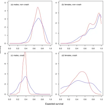
I predicted expected absolute fitness (survival) for each individual from the fitted glm and ridge 302
regression models. The distributions of expected absolute fitness are shown in figure 2. This 303
provides a overall picture of the amount of variation in fitness that is associated with regression-304
based inference about selection. The distributions of expected fitness from the glm, suggests that 305
on the basis of just four traits out of the entire multivariate phenotype, one could essentially 306
predict death or survival for many individuals with near certainty. On the other hand, the ridge 307
regression represents a seemingly more appropriately modest inference of the predictive power 308
of a handful of traits. This does not demonstrate that the non-regularised regression analysis is 309
have more reasonable interpretations for some purposes. 311
2.6 Selection of major axes of P 312
An alternative and common (e.g., Bolnick & Lau 2008; Grether 1996; Schluter & Smith 1986) 313
means of reducing the dimensionality of a selection analysis is to consider only the relationship 314
between major axes of phenotypic variation and fitness. For each dataset, I applied a spectral 315
decomposition of the phenotypic correlation matrix, and then rotated the phenotypic data onto 316
the two largest axes (largest eigenvalues) of P. Specifically, given the first two eigenvectors
317
of the distribution of phenotype, L2, and the original phenotypic records z, the new ‘traits’
318
representing loadings of the first two major axes of phenotype are z2 = zL2. I then estimated
319
selection gradients ofz2 by first fitting a glm with linear, quadratic and interaction terms, and
320
then obtained selection gradients from this function, as above, and also generated standard errors 321
and applied statistical hypothesis tests using the parametric bootstrap. Variance-standardised 322
selection gradient estimates pertaining to the major axes of P are given in table 5. These
323
estimates are interpretable as the selection intensities of the main axes of phenotype as defined 324
by the correlation structure of the traits. A variety of other standardisations are possible. Each 325
would require di↵erent interpretation, and each may reveal di↵erent information about natural
326
selection. 327
In these datasets, estimating selection of compound axes of phenotype does not provide very 328
meaningful inference of multivariate selection. In the example analyses, this practice revealed a 329
pattern of “bigger is better” across all traits, i.e., there would appear to be positive selection of 330
an axis onto which all three of the morphometric traits load positively. This fails to elucidate 331
patterns that are otherwise easily obtained (tables 2 and 4). In particular, the “bigger is better” 332
result that arises from analysis of principle components of phenotype conflicts with two important 333
findings: (i) Mass, rather than structural size is more proximally related to fitness, certainly in 334
non-crash years, and probably overall, and (ii) while large horns appear to be positively selected 335
via their loading of the directionally selected first ‘size’ axis of phenotype, horns are probably 336
2.7 (Generalised) projection-pursuit regression-based selection gradients and fit-338
ness surface estimation 339
The use of projection-pursuit regression (Friedman & Stuetzle, 1981) to estimate fitness functions 340
has been little-used since its introduction to the field by Schluter & Nychka (1994). This method 341
reduces the dimensionality of the problem by seeking the orthogonal axes of the multivariate 342
phenotype that maximise the explained variation in fitness. Each axis is characterised by a ridge 343
function, typically characterised by a semi-parametric smooth regression function. Briefly, the 344
response variable (or its linear predictor) is modelled aslink(E[y]) =µ+Pki fi(biX) +ei, where
345
fi() are the ridge functions associated with the estimated axes of phentoype that best explainy,
346
as defined by b; in the notation employed here for fitness functions, y=W and X =z. Both b
347
and the parameters of the arbitrary ridge functions fi() are estimated, simultaneously yielding
348
inference of the axes of phenotype that are selected, and of the form of selection. A complete 349
description of the method, with specific application to inference of fitness functions, is given in 350
Schluter & Nychka (1994). 351
I implemented a generalised projection-pursuit function (gppr) by wrapping the function 352
ppr(), in the R package stats in an iterative re-weighting function. I used cubic regression
353
spline regressions fitted by generalised cross validation for the ridge functions (matching the 354
implementation by Schluter & Nychka 1994). I characterised each fitness function with gppr 355
functions with one and two main axes. As above, I extracted selection gradient estimates from 356
the inferred fitness functions following Morrissey & Sakrejda (2013). The gppr function,gppr(), 357
and a function to obtain selection gradients from gppr analysis,gppr.gradients(), are included
358
in version 2.0 of the R package gsg (originally described in Morrissey & Sakrejda 2013). I
359
obtained estimates of the selection gradients of the major axes of selection as determined by 360
gppr by rotating the phenotypic data onto the axes identified in the gppr analysis, and then 361
refitting the model using gam() in mgcv, with univariate splines for each axis. I then recovered
362
the selection gradients of these axes usinggam.gradients() in gsg.
363
Because familiar hypothesis testing is not directly compatible with models fitted by cross-364
explained by the gppr models, over and above statistical noise. I made 1000 datasets for each 366
sex and environmental condition, each with the available sample size and observed distribution 367
of phenotype, but with randomised survival records. I then applied the gppr analyses with 368
one and two ridge functions, predicted individual absolute fitness for each fit, and recorded the 369
variance in predicted absolute fitness for each fitted function for each randomised dataset. I then 370
compared the variance in predicted absolute fitness, and the di↵erences in predicted absolute
371
fitness between models with one and two dimensions, between the randomised datasets and the 372
real datasets. 373
The gppr analyses revealed largely directional and linear selection (figure 3). The only sug-374
gestion of curvature of the major axes of selection was for females in non-crash years, and is more 375
interpretable as expected fitness asymptotically approaching one, rather than any mechanism of 376
non-linear selection. Because selection appears to be largely linear, the loadings of phenotype 377
onto the major axis of selection closely matched estimated directional selection gradients (table 378
2b). 379
In all cases, one axis of phenotype explained substantial variation in fitness (table 6). For all 380
analyses, I plotted the first major axis for ease of interpretation (figure 3); for males in non-crash 381
years, the predictions based on two axes were not interpretable in terms of any simple pattern 382
of selection. The gppr functions with two dimensions of selection did not explain much more 383
variation than the replicated analyses of randomised datasets (table 6), except for males in non-384
crash conditions; however, in that case, the amount of additional explained variation associated 385
with the two dimension model was nonetheless modest. 386
2.8 Supplementary simulations
387
For better or worse, the primary approach in this study was to compare the inferences that 388
could be made by applying di↵erent types of regression-based selection analyses to the same
389
empirical datasets. For better, consideration of the behaviour of the di↵erent analyses in their
390
application to real data has revealed a number of phenomena that might not otherwise have 391
surfaced. For worse, it is rarely possible to determine with certainty which analyses are most 392
clear whether and which phenomena that have occurred in the specific analyses here will be 394
important in general. While the purpose here is not to conduct any comprehensive simulation 395
studies, two specific issues seem to necessitate a little further investigation. These and other 396
issues would certainly benefit from more comprehensive studies. 397
2.8.1 Regularised regression analyses
398
The application of ridge regression, the lasso, and the elastic net regression to the Soay sheep 399
lamb datasets did not reveal any major benefits relative to other methods. One reason for this 400
may be that the dimensionality of the selection analysis problems in this study are rather low, 401
i.e., four traits. Combined with the fact that the ecological relevance of each trait is reasonably 402
intuitive to a human, we are inclined to think about selection on a trait-by-trait basis. It would be 403
a shame if the potential benefits of these analyses were marginalised because their benefits are not 404
immediately apparent in a single case study. One major potential benefit of regularised regression 405
is that it should be expected to provide some reduction in the tendency for statistical noise to 406
generate biases in some geometric properties of selection gradients, in particular, in the total 407
length of ˆ . If evolutionary quantitative genetic studies are able to become more multivariate, 408
and are able to apply geometric concepts to understanding evolution, as advocated for example 409
by Blows (2007) and Walsh & Blows (2009), robust inference of geometric properties of quantities 410
such as selection gradient vectors and G matrices will become increasingly important. Here, I
411
continue with the idea from the introduction that the norm of ˆ may be a very biased estimator 412
of|| ||, and test more generally by simulation whether regularised regression can provide better 413
inference. In geometric interpretations of microevolutionary parameters, || || is just one of
414
several important geometric quantities, appearing, for example, in theoretically well-justified 415
metrics of evolutionary constraint (Hansen & Houle, 2008). 416
I simulated 24 di↵erent scenarios, including every combination of: (i) sample sizes of n=100,
417
200, and 500 individuals, (ii) number of trait, k = 4, 10, (iii) normal (µ=0, =0.5) and
t-418
distributed (µ=0, =0.5, df=1) logistic scale regression gradients of expected fitness (i.e., W
419
in [0,1]), and (iv) low and high dispersion of eigenvalues of the P matrix. For each simulation,
420
unique P matrices were simulated from an inverse Wishart distribution of V=I, and ⌫ = 20
and 5, when k = 4 for low and high dispersion of P, respectively, and ⌫ = 30 and 11, when 422
k = 10 for low and high dispersion of P. Each P matrix was standardised to unit variance
423
in each trait. For each simulation, I simulated n records of k traits, z, with mean vectors of
424
0, and covariance P. For each simulation I also drew unique logistic scale gradients of fitness 425
with respect to phenotype,b, according to either the normal or t-distribution, depending on the
426
scenario. I then simulated individual fitness records from a binomial distribution with expected 427
value logit 1(zb0).
428
I calculated the resulting true selection gradients by a modification of the Morrissey & Sakre-429
jda (2013) algorithm. I generated 106 records of phenotype according to the true value of P
430
for each replicate simulation. For each phenotypic record, I then calculated expected absolute 431
fitness, and averaged these to obtain population mean expected fitness. Then, separately for 432
each of thek traits, I re-calculated population mean fitness for a modified dataset in which 0.03
433
had been added to each phenotypic record for a given trait, and repeated with subtracting 0.03. 434
I then calculated the partial derivative of population mean fitness with respect to phenotype, 435
scaled to relative fitness, i.e., the selection gradient, for each trait, by finite di↵erences. I re-436
peated this algorithm five times for each replicate of each simulation scenario. Values of the true 437
values of agreed to the 4th decimal place in most replicate applications of the MC procedure.
438
I took the means across the five simulations to be the true values of .
439
I then applied logistic regression analyses with linear terms only in each replicate simulation 440
scenario. I fitted GLMs, as well as ridge, lasso, and elastic ridge regressions, and in each case 441
obtained selection gradient estimates, as described above for the case studies in Soay sheep. In 442
each replicate simulation I calculated |||| ||ˆ|| for each of the four regression-based estimates of ˆ . As 443
predicted by the simple theory developed in the introduction and the appendix, the estimates 444
of the total magnitude of selection are upwardly biased in analyses non-regularised analyses, 445
especially when the P matrix is ill-conditioned (figure 4). Regularised regression analyses yield
446
somewhat negatively, but less, biased inference of || ||. The analyses also reveal that the best
447
2.8.2 Major axes of selection
449
I further investigated the degree to which the inference of the major axes of estimated matrices
450
is biased toward minor axes of the phenotype by simulating eight di↵erent scenarios of bivariate
451
quadratic selection analyses, involving high and modest phenotypic correlations (r = 0.8 and
452
0.5), two sample sizes (n = 250 and 500), and for no selection, and for true stabilising selection
453
on one trait (fitness function was binomial with logit(E(W|zi)) = 0.3z2i). The simulations
454
with true stabilising selection thus had a true angle between the major axes of P and of 45
455
degrees. 456
The null distribution of the direction of the major axis of quadratic selection, relative to the 457
major axis of phenotype, is highly biased toward orthogonality, especially when there are strong 458
phenotypic correlations between traits (figure 5a,c). Even when selection occurs, substantial 459
bias of estimated major axes of selection occurs (figure 5b). In the best case scenario, with sub-460
stantial (true) selection which is easily characterised because of modest phenotypic correlations, 461
inferences based on rotation of estimated matrices can become robust (figure 5d). In the
462
context of multivariate selection analyses, even when correlations as high as 0.8 do not occur, 463
similarly minor axes of phenotype to the simulations in figure 5a,b are common. Consequently, 464
it seems that substantial biases in the direction of major axes of relative to Pare likely to be
465
prevalent in most studies of multivariate non-linear selection. 466
3
Discussion
467
Exploration of a broad range of regression analyses for quantitative inferences of natural selec-468
tion revealed useful properties of several under-used approaches, and also illustrated important 469
limitations of some commonly applied analyses. In particular, two previously unacknowledged 470
properties of diagonalised quadratic selection matrices seriously hinder interpretation: (i) the 471
method is biased toward apparent detection of quadratic selection that is orthogonal to major 472
axes of variation, and (ii) biases aside, the magnitudes of the major axes of variance-standardised 473
cannot be interpreted in variance-standardised units. However, in conjunction with recently 474
tions (Morrissey & Sakrejda, 2013), projection-pursuit regression may be able to serve for the 476
main biological questions for which diagonalisation of has been suggested, and will also
pro-477
vide other useful properties. More generally, quantitative inference of selection gradients from 478
arbitrary regression analyses will allow useful properties of a greater range of types of selection 479
analysis to be exploited for the study of natural selection. 480
In the example datasets, several conclusions are repeatedly supported by di↵erent analyses.
481
First, while larger size is generally selected, mass is more directly associated with first winter 482
survival than is structural size, as represented here by leg length. The positive direct selection 483
of mass reported here does not contradict the previously reported associations of limb length 484
with neonatal survival Coltman et al. (1999), as the lack of direct e↵ect characterised by the
485
selection di↵erential (low here for leg length; table 2b) neither precludes association (table 2a), 486
or an indirect mechanistic e↵ect of leg length on survival. The strong direct e↵ect of mass is
487
supported by all regression-based inferences of selection gradients, although the pattern is more 488
tenuous in crash rather than non-crash years, and also coincides with extensive work showing 489
associations of mass with life history in this population (Milneret al., 1999). While it is probably 490
not possible to conclude that mass-fitness relationships, in adults at least, are causal (Morrissey 491
et al., 2012a), it seems plausible that energy reserves in lambs could well be a key causal variable
492
in determining first winter survival. It appears that for crash years, smaller available sample 493
sizes combined with high covariances among traits conspire to make separation of direct and 494
indirect e↵ects very difficult. The regularised regression analyses, particularly the lasso, which 495
allows some degree of inherent variable selection, suggest that the pattern of mass, rather than 496
structural size, being most proximal to survival, may hold in crash years as well (table 4). 497
Whereas there is either little selection, or positive selection,of horn size in lambs across sexes 498
and environmental conditions (i.e., near zero or positive selection di↵erentials), there appears to 499
be substantial selectionfor (terminology for association vs. e↵ect following Sober 1984) smaller 500
horn size in non-crash years. The pattern in non-crash years, at least, is simple and intuitive, as 501
investment in horns is unlikely to positively influence survival in general (Johnstonet al., 2013; 502
Robinson et al., 2006) or survival of lambs in particular. I am hesitant to interpret estimated
503
variation in selection, as uncertainty in their estimation precludes rejection of the possibility of 505
similar selection across environmental conditions. If indeed selection does directly favour horn 506
size, at least directly with reference to the traits studied here, this could reflect utility of horns 507
for competition for scarce resources. 508
The simple “bigger is better” pattern apparently revealed by positive selection of the first 509
axis on phenotypic variation gives an impression of simple directional selection on the traits 510
underlying the first axis (mass, leg length, and horn length), in both sexes and environmental 511
conditions. All other analyses show that this pattern does not reflect reality, at least not in 512
non-crash years where direct e↵ects of traits can be estimated with relative precision. Certainly, 513
situations will arise where principle components will reflect ecologically-relevant axes of varia-514
tion. However, the analyses here highlight that statistically dominant and ecologically important 515
axes of variation may be very di↵erent. At the very least, results of selection analyses of prin-516
ciple components should be approached with caution, especially when the motivation for using 517
principle components is statistical (dimensionality reduction), rather than biological. 518
Regularised regression methods (i.e., the lasso, ridge regression, and the elastic net) generally 519
supported patterns in selection gradients that were obtained from more traditional regression-520
based analyses. The lasso may have provided improved inferences in cases where trait covariances 521
otherwise precluded inference of selection gradients. For example, it is useful that the lasso 522
was able to identify a most-probable proximate e↵ect of mass on survival in males in crash
523
years, where other methods were essentially unable to distinguish among potential e↵ects of the
524
di↵erent traits. Similarly, the total amounts of variation in survival that are apparently explained 525
by regression analyses (figure 2) are much more plausible for ridge, rather than for (unpenalised) 526
least-squares regression. While the application of these regularised regression analyses did not 527
greatly help interpretation of the Soay sheep example data, it is possible that they could be quite 528
useful in other circumstances, especially for making geometric interpretations about multivariate 529
selection (figure 4). 530
Two major features of the analyses of multivariate non-linear selection in the Soay sheep lamb 531
datasets highlight the difficulties in interpretation of the major axes of the quadratic selection 532
gradient matrix, . It may initially seem quite bold to criticise existing methods for analysis
of non-linear selection based on example analyses of datasets that do not, it turns out, seem 534
to contain much non-linear selection. However, the undesirable behaviours of inferences about 535
the estimated matrix here will exist in any analysis, regardless of the underlying reality. The
536
first serious problem is that statistical noise has a very insidious e↵ect on the orientation of the 537
estimated major axes of . The true curvature of will be hardest to estimate in directions
538
within P that have the least variance. Therefore, major axes of are likely to correspond to
539
minor axes of phenotype, purely as an artefact of the fact that statistical noise will create the 540
greatest estimated values in directions within P that have the least variance. Such a pattern
541
unfortunately has a very tempting biological interpretation, i.e., that quadratic selection and 542
multivariate phenotype are aligned. This problem is quite intuitive once one starts to consider 543
the e↵ect of noise on a table of estimated selection coefficients such as . Note that this problem 544
will a↵ect all axes of estimated matrices, influencing both shape and orientation. Even where
545
axes exist that are subject to quadratic selection, inference of their orientation will be hindered 546
by the fact that the orientation of other axes is biased by the shape of P, combined with the
547
constraint of orthogonality inherent to diagonalisation (table 5). This problem arises because 548
of di↵erent amounts of variation in di↵erent directions of phenotypic space. Therefore, it will 549
a↵ect analyses of major axes of matrices under any system of trait standardisation.
550
A second difficulty with spectral decomposition of is specific to analysis of
variance-551
standardised matrices. Where the original gradients are interpretable as the direct components
552
of selection intensities, i.e., they reflect the amount of fitness variation directly associated with 553
(quadratic) selection of the traits, given the standing variation in the traits, the major axes of 554
gamma do not have this interpretation. This phenomenon is particularly noticeable in figure 1b. 555
Here, the most curved direction of is aligned with an axis ofP(table 1) that has little variation 556
(whether this is real, or chance, is not immediately relevant to this second point). Consequently, 557
the first axis of stabilising selection is actually associated with less variation in fitness than the 558
second axis! This is apparent in figure 1b, where the curvature of the second axis is indeed 559
less than that of the first, but it represents stronger selection because it is associated with more 560
phenotypic variation. 561
remains extremely important. Fortunately, a variety of features of projection-pursuit regression 563
make it highly amenable to the study of multivariate selection. In combination with methods to 564
obtain quantitatively interpretable selection gradients from projection-pursuit regression-based 565
inferences of fitness functions, as applied here, this method can probably supplant the practice 566
of diagonalisation of . The first major empirical benefit of projection-pursuit regression is that 567
it can be used to seek the major axes of selection, not just the major axes of directional or of 568
quadratic selection. In addition to the issues already discussed about diagonalisation of , there 569
has never been any real resolution to the fact that quadratic univariate or multivariate selection, 570
considered either in isolation or in conjunction with , does not address key biological questions 571
about natural selection, such as whether or not fitness optima exist (Schluter, 1988). gppr, on 572
the other hand, provides a method of characterising the major axes of selection, whether they 573
be linear, disruptive, stabilising, or purely directional but curved. Further investigations of the 574
behaviour of gppr-based selection analysis seems warranted, as it is currently unknown what 575
e↵ects details of its application, for example the form of ridge functions, may have on inferences 576
of selection. 577
Reporting of maximum likelihood estimates of selection coefficients, i.e., such as those
com-578
monly reported to date and in table 2, will remain very important. These, and associated 579
information about their statistical uncertainties, are required for meta analysis. To date, failure 580
to report standard errors has severely limited sample sizes in formal meta-analyses of selection 581
(Morrissey & Hadfield, 2012; Siepielskiet al., 2013). However, reporting standard errors is only 582
a start. Reporting of sampling variances and covariances, in additional to full reporting of sum-583
mary statistics, will also be very useful. Sampling covariances could potentially be reported by 584
archiving posterior distributions, or bootstrap samples, of fitted models of fitness functions. An 585
efficient way to report full distributions of sampling variance may be to archive bootstrap
dis-586
tributions of selection coefficients, such as those that are generated automatically by functions 587
in theR package gsg (Morrissey & Sakrejda, 2013).
Conclusion 589
The availability of an approach to obtain valid inference of selection gradients from arbitrary 590
regression-based inferences of fitness functions renders a large range of techniques available for 591
quantitative inference of natural selection. I have explored a range of these methods, and dis-592
sected some key aspects of the behaviour of each. Projection-pursuit regression seems to stand 593
out as a method for characterisation of multivariate selection. Its greater use will facilitate on-594
going attempts to implement multivariate quantitative genetic studies on selection in natural 595
populations and experimental systems. Furthermore, identification of major axes of selection, as 596
opposed to major axes of directional or quadratic selection, will bring much more direct biological 597
interpretation to multivariate selection analysis. 598
4
Acknowledgements
599
Josephine Pemberton and Loeske Kruuk provided valuable comments on an earlier version of 600
this manuscript. The manuscript also benefited greatly from input by Thomas Hansen, Bruce 601
Walsh, and an anonymous reviewer. Jarrod Hadfield suggested that the secondary theorem-602
based proof in the appendix might be most convincing, and Len Thomas, Ian Goudie, and Peter 603
Jupp provided the proof. The Soay sheep data were provided by Josephine Pemberton and 604
Loeske Kruuk, and were collected primarily by Jill Pilkington and Andrew MacColl with the 605
help of many volunteers. The collection of the Soay sheep data is supported by the National 606
Trust for Scotland and QinetQ, with funding from NERC, the Royal Society, and the Leverhulme 607
Trust. 608
5
Appendix
609
Denote an arbitrary function relating trait to relative fitness, w(z), and a decomposition of an
610
individual i’s trait value, z, into e↵ects of breeding value and environment zi =ai+ei Assume
611
that a and e are independent, ai ⇠ p(a) and ei ⇠ q(e), such that the variance of phenotype
612
in a population obeys 2
z = a2+ e2. Assume that p(a) represents a normal probability density
613
function with mean zero and variance 2
a, such that p(a) = ap12⇡e a2
2 2a, and that q(e) is an
614
The secondary theorem (Robertson, 1966) defines 616
¯
z = a,w, (A1)
which by definition is 617
¯
z =E(a·w) E(a)E(w). (A2)
The second term in A2 is zero because theE(a) is zero by construction. So, from equation A2,
618
¯
z =
Z 1
1
a
Z 1
1
w(a+e)p(a)q(e)deda. (A3)
The average slope of the relative fitness function, w0(z), given normally distributed breeding
619
values and conditioning one, can be writtenR11w0(a+e)p(a)da. p0(a) = a2
ap(a), so integration
620
by parts gives 621
Z 1
1
w0(a+e)p(a)da= [w(a+e)p(a)] +
Z 1
1
w(a+e) a2
a
p(a)da
=
Z 1
1
w(a+e) a2
a
p(a)da.
(A4)
The simplification assumes that the relative fitness function is bounded. Applying Fubini’s 622
theorem to the double integral and multiplying equation A3 by 2a
2
a, and then substituting using
623
equation A4 gives 624
¯
z =
Z 1
1
Z 1
1
2
aw(a+e)
a
2 a
p(a)q(e)dade,
=
Z 1
1
Z 1
1
2
aw0(a+e)p(a)q(e)dade,
= 2a
Z 1
1
Z 1
1
w0(a+e)p(a)q(e)dade.
(A5)
So, evolution of the mean phenotype is given by the variance of normally distributed breeding 625
values, times the average slope of the relative fitness function integrated over the distribution of 626
phenotype, regardless of the distribution of environmental e↵ects on phenotype.
627
6
Data accessibility
628
R functions and example datasets are included in an update to the R package gsg.
629
References
630
Bell, G. (2010) Fluctuating selection: the perpetual renewal of adaptation in variable environ-631
ments. Philosophical Transactions of the Royal Society, Series B,365, 87–97.
Blows, M.W. (2007) A tale of two matrices: multivariate approaches in evolutionary biology. 633
Journal of Evolutionary Biology,20, 1–8.
634
Bolnick, D.I. & Lau, O.L. (2008) Predictable patterns of disruptive selection in stickleback in 635
postglacial lakes. The American Naturalist, 172, 1–11.
636
Carlson, S.M. & Quinn, T.P. (2007) Ten years of varying lake level and selection on size-at-637
maturity in sockeye salmon. Ecology, 88, 2620–2629.
638
Clutton-Brock, T.H. & Pemberton, J.M. (2004)Soay sheep dynamics and selection in an island
639
population. Cambridge University Press, Cambridge.
640
Clutton-Brock, T.H., Price, O.F., Albon, S.D. & Jewell, P.A. (1992) Early development and 641
population fluctuations in soay sheep. Journal of Animal Ecology,61, 381–396.
642
Coltman, D.W., Smith, J.A., Bancroft, D.R., Pilkington, J., MacColl, A.D.C., Clutton-Brock, 643
T.H. & Pemberton, J.M. (1999) Density-dependent variation in lifetime breeding success and 644
natural sexual selection in soay rams. The American Naturalist, 154, 730–746.
645
Dickerson, G.E. (1955) Genetic slippage in response to selection for multiple objectives. Cold
646
Spring Harbor Symposia on Quantitative Biology, 20, 213–224.
647
Dormann, C.F., Elith, J., Bacher, S., Buchmann, C., Carl, G., Carr´e, G., Marqu´ez, J.R.G., Gru-648
ber, B., Lafourcade, B., ao, P.J.L., M¨unkem¨uller, T., McClean, C., Osborne, P.E., Reineking, 649
B., Schr¨oder, B., Skidmore, A.K., Zurell, D. & Lautenbach, S. (2013) Collinearity: a review of 650
methods to deal with it and a simulation study evaluating their performance. Ecography,36,
651
27–46. 652
Endler, J.A. (1986)Natural selection in the wild. Princeton University Press.
653
Engen, S. & Saether, B.E. (2014) Evolution in fluctuating environments: decomposing selection 654
into additive components of the Robertson-Price equation. Evolution, 68, 854–865.
655
Engen, S., Saether, B.E., Kvalnes, T. & Jensen, H. (2012) Estimating fluctuating selection in 656
age-structured populations. Journal of Evolutionary Biology, 25, 1487–1499.
Friedman, J., Hastie, T. & Tibshirani, R. (2008) Regularization paths for generalized linear 658
models via coordinate descent. Journal of Statistical Software,33, 1–22.
659
Friedman, J.H. & Stuetzle, W. (1981) Projection pursuit regression. Journal of the American
660
Statistical Association,76, 817–823.
661
Geyer, C.J., Wagenius, S. & Shaw, R.G. (2007) Aster models for life history analysis.Biometrika, 662
94, 415–426. 663
Grant, P.R. & Grant, B.R. (2002) Unpredictable evolution in a 30-year study of Darwin’s finches. 664
Science, 296, 707–711.
665
Grether, G.F. (1996) Sexual selection and survival selection on wing coloration and body size in 666
the rubyspot damselfly Hataerina americana. Evolution, 50, 1939–1948.
667
Hansen, T.F. & Houle, D. (2008) Measuring and comparing evolvability and constraint in mul-668
tivariate characters. Journal of Evolutionary Biology, 21, 1201–1219.
669
Hereford, J., Hansen, T.F. & Houle, D. (2004) Comparing strengths of directional selection: how 670
strong is strong? Evolution, 58, 2133–2143.
671
Johnston, S.E., Gratten, J., Berenos, C., Pilkington, J.G., Clutton-Brock, T.H., Pemberton, 672
J.M. & Slate, J. (2013) Life history trade-o↵s at a single locus maintain sexually selected 673
genetic variation. Nature, 502, 93–95.
674
Kingsolver, J.G., Hoekstra, H.E., Hoekstra, J.M., Vignieri, C., Berrigan, D., Hill, E., Hoang, A., 675
Gilbert, P. & Beerli, P. (2001) The strength of phenotypic selection in natural populations. 676
The American Naturalist, 157, 245–261.
677
Lande, R. & Arnold, S.J. (1983) The measurement of selection on correlated characters.
Evolu-678
tion,37, 1210–1226. 679
Lockhart, R., Taylor, J., Tibshirani, R.J. & Tibshirani, R. (2013) A significance test for the 680
lasso. available at http://arxivorg, arXiv:1301.7161v2.
681
MacColl, A.D.C. (2011) The ecological causes of evolution. Trends in Ecology and Evolution,
682
Milner, J.M., Albon, S.D., Illius, A.W., Pemberton, J.M. & Clutton-Brock, T.H. (1999) Repeated 684
selection of morphometric traits in the Soay sheep of St Kilda. Journal of Animal Ecology,68,
685
472–488. 686
Mitchell-Olds, T. & Shaw, R.G. (1987) Regression analysis of natural selection: statistical infer-687
ence and biological interpretation. Evolution,41, 1149–1161.
688
Morrissey, M.B. (2014) Selection and evolution of causally covarying traits. Evolution,68, 1748–
689
1761. 690
Morrissey, M.B. (in review) Severe biases in synthetic meta-analyses that fail to account for the 691
observation process. The American Naturalist.
692
Morrissey, M.B. & Hadfield, J.D. (2012) Directional selection in temporally replicated studies is 693
remarkably constant. Evolution, 66, 435–442.
694
Morrissey, M.B., Parker, D.J., Korsten, P., Pemberton, J.M., Kruuk, L.E.B. & Wilson, A.J. 695
(2012a) The prediction of adaptive evolution: empirical application of the secondary theorem 696
of selection and comparison to the breeder’s equation. Evolution, currently online early.
697
Morrissey, M.B. & Sakrejda, K. (2013) Unification of regression-based approaches to the analysis 698
of natural selection. Evolution,67, 2094–2100.
699
Morrissey, M.B., Walling, C.A., Wilson, A.J., Pemberton, J.M., Clutton-Brock, T.H. & Kruuk, 700
L.E.B. (2012b) Genetic anlaysis of life history constraint and evolution in a wild ungulate 701
popualtion. American Naturalist, 179, E97–E114.
702
Philips, P.C. & Arnold, S.J. (1989) Visualizing multivariate selection. Evolution,43, 1209–1222. 703
Plummer, M. (2010)JAGS version 2.0 Manual. International Agency for Research on Cancer.
704
Poissant, J., Wilson, A.J., Festa-Bianchet, M., Hogg, J.T. & Coltman, D.W. (2008) Quantitative 705
genetics and sex-specific selection on sexually dimorphic traits in bighorn sheep. Proceedings
706
of the Royal Society, B Series, 275, 623–628.
Reynolds, R.J., Childers, D.K. & Pajewski, N.M. (2010) The distribution and hypothesis testing 708
of eigenvalues from the canonical analysis of the gamma matrix of quadratic and correlational 709
selection gradients. Evolution, 64, 1076–1085.
710
Rice, W.R. (1989) Analysing tables of statistical tests. Evolution, 43, 223–225.
711
Robertson, A. (1966) A mathematical model of the culling process in dairy cattle. Animal
712
Production, 8, 95–108.
713
Robinson, M.R., Pilkington, J.G., Clutton-Brock, T.H., Pemberton, J.M. & Kruuk, L.E.B. 714
(2006) Live fast, die young: a balance of natural, sexual and antagonistic selection maintains 715
phenotypic polymorphism of weaponry in male and female soay sheep. Evolution, 60, 2168–
716
2181. 717
Ro↵, D.A. & Fairbairn, D.J. (2007) The evolution of trade-o↵s: where are we? Journal of
718
Evolutionary Biology, 20, 433–447.
719
Schluter, D. (1988) Estimating the form of natural selection on a quantitative trait. Evolution,
720
42, 849–861. 721
Schluter, D. & Nychka, D. (1994) Exploring fitness surfaces. The American Naturalist, 143,
722
597–616. 723
Schluter, D. & Smith, J.N.M. (1986) Natural selection on beak and body size in the song sparrow. 724
Evolution, 40, 221–231.
725
Shaw, R.G. & Geyer, C.J. (2010) Inferring fitness landscapes. Evolution,64, 2510–2520.
726
Siepielski, A.M., DiBattista, J.D. & Carlson, S.M. (2009) It’s about time: the temporal dynamics 727
of phenotypic selection in the wild. Ecology Letters,12, 1261–1276.
728
Siepielski, A.M., Gotanda, K.M., Morrissey, M.B., Diamond, S.E., DiBattista, J.D. & Carlson, 729
S.M. (2013) The spatial patterns of directional phenotypic selection. Ecology Letters.
730
Sober, E. (1984) The Nature of Selection. University of Chicago Press, Chicago.
Tibshirani, R. (1996) Regression shrinkage and selection via the lasso. Journal of the Royal
732
Statistical Society, Series B,58, 267–288.
733
Tikhonov, A.N. & Arsenin, V.Y. (1977) Solution of ill-posed problems. Winston and sons,
734
Washington. 735
Walsh, B. & Blows, M.W. (2009) Abundant genetic variation + strong selection = multivariate 736
genetic constraints: a geometric view of adaptation. Annual Review of Ecology, Evolution,
737
and Systematics,40, 41–59.
738
Wilson, K., Grenfell, B.T., Pilkington, J.G., Boyd, H.E.G. & Gulland, F.M.D. (2004) Parasites
739
and their impact, in Soay sheep: dynamics and selection in an island populaiton, T. H.
Clutton-740
Brock and J. M. Pemberton, eds. Cambridge University Press.
741
Wood, S.N. (2006) Generalized Additive Models: An Introduction with R. Chapman and
742
Hall/CRC. 743
Zou, H. & Hastie, T. (2005) Regularization and variable selection via the elastic net. Journal of
744
the Royal Statistical Society, Series B, 67, 301–320.