Improving the efficiency of learning CSP solvers

(1)

IMPROVING THE EFFICIENCY OF LEARNING CSP SOLVERS

Neil C.A. Moore

A Thesis Submitted for the Degree of PhD at the

University of St. Andrews

2011

Full metadata for this item is available in Research@StAndrews:FullText

at:

http://research-repository.st-andrews.ac.uk/

Please use this identifier to cite or link to this item:

http://hdl.handle.net/10023/2100

(2)

Improving the efficiency of learning CSP solvers

Thesis by

Neil C.A. Moore

In Partial Fulfillment of the Requirements

for the Degree of

Doctor of Philosophy

University of St Andrews

School of Computer Science

(3)

Abstract

Backtracking CSP solvers provide a powerful framework for search and reasoning.

The aim of constraint learning is increase global reasoning power by learning new

constraints to boost reasoning and hopefully reduce search effort. In this thesis

con-straint learning is developed in several ways to make it faster and more powerful.

First, lazy explanation generation is introduced, where explanations are generated

as needed rather than continuously during propagation. This technique is shown

to be effective is reducing the number of explanations generated substantially and

concequently reducing the amount of time taken to complete a search, over a wide

selection of benchmarks.

Second, a series of experiments are undertaken investigating constraint forgetting,

where constraints are discarded to avoid time and space costs associated with

learn-ing new constraints becomlearn-ing too large. A major empirical investigation into the

overheads introduced by unbounded constraint learning in CSP is conducted. This is

the first such study in either CSP or SAT. Two significant results are obtained. The

first is that typically a small percentage of learnt constraints do most propagation.

While this is conventional wisdom, it has not previously been the subject of

empiri-cal study. The second is that even constraints that do no effective propagation can

incur significant time overheads. Finally, the use of forgetting techniques from the

literature is shown to significantly improve the performance of modern learning CSP

solvers, contradicting some previous research.

Finally, learning is generalised to use disjunctions of arbitrary constraints, where

before only disjunctions of assignments and disassignments have been used in

prac-tice (g-nogood learning). The details of the implementation undertaken show that

major gains in expressivity are available, and this is confirmed by a proof that it can

(4)

ABSTRACT ii

save an exponential amount of search in practice compared with g-nogood learning.

(5)

Declaration

Only kings, presidents, editors, and

people with tapeworms have the

right to use the editorial ’we.’

Mark Twain

I, Neil C.A. Moore, hereby certify that this thesis, which is approximately 48381

words in length, has been written by me, that it is the record of work carried out

by me and that it has not been submitted in any previous application for a higher

degree.

Date . . . Signature of candidate . . . .

I was admitted as a research student in September 2007 and as a candidate for the

degree of Doctor of Philosophy in September 2008; the higher study for which this is

a record was carried out in the University of St Andrews between 2007 and 2010.

I hereby certify that the candidate has fulfilled the conditions of the Resolution and

Regulations appropriate for the degree of Doctor of Philosophy in the University of

St Andrews and that the candidate is qualified to submit this thesis in application

for that degree.

Date . . . Signature of supervisor . . . .

(6)

DECLARATION iv

In submitting this thesis to the University of St Andrews I understand that I am giving

permission for it to be made available for use in accordance with the regulations of the

University Library for the time being in force, subject to any copyright vested in the

work not being affected thereby. I also understand that the title and the abstract will

be published, and that a copy of the work may be made and supplied to any bona fide

library or research worker, that my thesis will be electronically accessible for personal

or research use unless exempt by award of an embargo as requested below, and that

the library has the right to migrate my thesis into new electronic forms as required

to ensure continued access to the thesis. I have obtained any third-party copyright

permissions that may be required in order to allow such access and migration, or have

requested the appropriate embargo below.

The following is an agreed request by candidate and supervisor regarding the

electronic publication of this thesis: Access to printed copy and electronic publication

of thesis through the University of St Andrews.

(7)

Copyright

In submitting this thesis to the University of St Andrews I understand that I am giving

permission for it to be made available for use in accordance with the regulations of

the University Library for the time being in force, subject to any copyright vested

in the work not being affected thereby. I also understand that the title and abstract

will be published, and that a copy of the work may be made and supplied to any

bona fide library or research worker, that my thesis will be electronically accessible

for personal or research use, and that the library has the right to migrate my thesis

into new electronic forms as required to ensure continued access to the thesis. I have

obtained any third-party copyright permissions that may be required in order to allow

such access and migration.

(8)

This is dedicated to my family and friends, but especially to those who never got a

(9)

Acknowledgements

I’d like to thank my supervisors, Ian Gent and Ian Miguel, for helping me to make the

transition from being told what to do to being an independent researcher. Thanks

to George Katsirelos for taking the time to give me detailed expert assistance at key

moments. Thanks to Chris Jefferson and Pete Nightingale for their patient help on

programming minion and understanding CP literature. Thanks to Patrick Prosser

for giving me an interest in constraints that has persisted ever since we met. Thanks

to Özgür Akgün, Andy Grayland, Lars Kotthoff, Yohei Negi and Andrea Rendl for

their help and companionship.

This research was funded by UK Engineering and Physical Sciences Research

Council (EPSRC) grant EP/E030394/1 named “Watched Literals and Learning for

Constraint Programming”.

(10)

Publications

I have had the following peer-reviewed articles in journals, international conferences

and workshops published during the course of this PhD. The first four entries are

based on work contained in this thesis and are all based upon my own work, the other

authors providing supervision and assistance with writing. The remaining entries are

work peripheral to the PhD in decreasing order of my contribution.

• I.P. Gent, I. Miguel, and N.C.A. Moore. Lazy explanations for constraint

propagators. In PADL 2010, number 5937 in LNCS, January 2010

• Ian P. Gent, Ian Miguel, and Neil C.A. Moore. An empirical study of

learn-ing and forgettlearn-ing constraints. In Proceedings of 18th RCRA International Workshop on ”Experimental Evaluation of Algorithms for solving problems with combinatorial explosion“, 2011

• Neil C.A. Moore. C-learning: Further generalised g-nogood learning. In Alan

Frisch and Barry O’Sullivan, editors, Proceedings of the ERCIM Workshop on Constraint Solving and Constraint Logic Programming, pages 103–119, 2011

• Neil C.A. Moore. Learning arbitrary constraints at conflicts. In Proceedings of the CP Doctoral Programme, September 2008

• Neil C.A. Moore. Propagating equalities and disequalities. In Proceedings of the CP Doctoral Programme, September 2009

• Neil Moore and Patrick Prosser. Species trees and the ultrametric constraint.

Journal of Artificial Intelligence Research, 32:901–938, 2008

• Christopher Jefferson, Neil C.A. Moore, Peter Nightingale, and Karen E.

Petrie. Implementing logical connectives in constraint programming. Artifi-cial Intelligence Journal (AIJ), 174:1407–1420, November 2010

(11)

PUBLICATIONS ix

• Ian P. Gent, Lars Kotthoff, Ian Miguel, Neil C.A. Moore, Peter Nightingale,

and Karen Petrie. Learning when to use lazy learning in constraint solving. In

Michael Wooldridge, editor, European Conference on Artificial Intelligence (ECAI), 2010

• Lars Kotthoff and Neil C.A. Moore. Distributed solving through model

(12)

Chapter 1 Introduction

This thesis is about the constraint satisfaction problem (CSP). The CSP has endur-ing practical appeal because it is a natural way of encodendur-ing problems that occur

spontaneously in practice. This is because the world is full of constraints, like credit

limits on bank accounts, the amount of shopping a person can carry and the force of

gravity. CSPs are useful because people may wish to know whether they can achieve

their aims subject to the constraints imposed on them, like whether there is a travel

itinerary visiting New York, London and Paris for under£1000.

So far, all I have done is to write down common sense since everyone copes

with constrainedness every day. However some problems of this type are extremely

difficult in practice, e.g. often finding a feasible school timetable is a difficult

un-dertaking due to the difficulty of reconciling shortage of space, time and

teach-ers. The idea of using computers to find solutions to such problems is very

at-tractive, imagining that they can try out thousands of combinations per second.

However even relatively simple looking practical problems can have huge numbers

of possible guesses and very few solutions that satisfy the constraints. Sudoku is

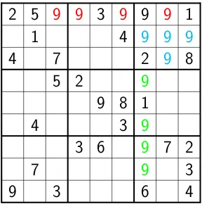
a CSP that many people are familiar with. The object of the game is to fill in

a grid (e.g. Figure 1.1) with numbers, such that each row, column and box

con-tains each number between 1 and 9. A sudoku has a single solution, but at most

11,790,184,577,738,583,171,520,872,861,412,518,665,678,211,592,275,841,109,096,961∗

com-plete assignments that are wrong! More formally, CSP is an NP-comcom-plete problem,

∗_{this is based on a sudoku with 17 clues: there are 64 remaining unknowns with 9 choices for}

each, hence 964 _{possible solutions}

(18)

1.1. CSP SOLVERS IN PRACTICE 2

so it is strongly suspected that no algorithm exists that can solve any CSP quickly

(in polynomial time).

In spite of the likely impossibility of finding a fast algorithm for CSP that works

in all cases, general purpose CSP solvers exist and are used to solve many problems in

practice. But why use a CSP solver, when you can write a solver just for timetabling,

or just for planning road trips? The reason is that general purpose solvers:

• incorporate the distilled wisdom of experts, e.g. efficient implementation and

effective general-purpose heuristics to help find a solution;

• adapt to solve variants of the original problem, something that a solver

tai-lored to one problem cannot easily do; and

• save programmer’s time because they can be taken off the shelf.

However, it is the burden of writers of CSP solvers to be constantly striving to

solve a larger range of instances, and faster, by incorporating clever new tricks into

their solver. In this thesis I attempt to do this for a certain type of CSP solver, as I

will now explain.

1.1. CSP solvers in practice

In this thesis, I will consider cases where the unknowns are integers and the constraints

may take any form, provided they are easy to check. For example, it is easy to verify a

solution to equationx2−2 = ym such thatx, y are integers and m≥3 by arithmetic, but it is an unsolved problem to find one (according to [Coh07]). Many commonly

used CSP solvers use a variation on backtracking search to find a solution. Typically they make a sequence of guesses to fill in unknowns, retracting decisions that don’t

lead to a solution and finishing when a solution is found or no more guesses are

possible. In this way every possible solution is eventually tried.

In its basic form this na¨ıve strategy can, for example, hit the worst case for

sudoku where 1.2×1061†_{different assignments are tried. One of the primary reasons}

why CSP solvers are able to be efficient in practice is that they integrate reasoning

algorithms for each constraint individually into backtracking search. For example,

consider the sudoku shown in Figure 1.1. The coloured numbers can be inferred to be

(19)

1.1. CSP SOLVERS IN PRACTICE 3

2 5

9 9

3

9

1

4 9 9 9

4

7

2

9

8 5 2

9 9 8 1

4

3

9 3 6

9 7 2

7

9

3

[image:19.595.157.445.73.363.2]

9

3

6

4

Figure 1.1. Example sudoku grid, clues are printed in black,

impos-sible entries in colour

impossible because of the (black) 9 already assigned. The red values are impossible

by reasoning with the constraint over the first row: no duplicate 9s are allowed.

The blue values are impossible by the constraint over the top-right box. Finally

the green values are ruled out by the constraint over the 7th column. This type of

simple reasoning has drastically cut the number of possible assignments, removing

284,294,103,884,805,425,687,795,982,353,378,114,796,118,426,545,7051

or 75% of the

possible assignments straight away! In general-purpose CSP solvers with this type

of “all different” reasoning can solve almost all sudokus very easily, however creating

hard sudoku puzzles by computer is still a challenging problem. The process of

removing values from consideration by inference is known as propagation.

Propagation is important to CSP solvers because it allows separation of concerns:

specialised inference algorithms are added in a controlled way, because there is one

for each constraint. There is no need to consider, for example, what to do with

combinations, such as x+y = z s.t. x 6= y. The solver simply has one algorithm

(20)

1.2. HYPOTHESES ON LEARNING IN CSP SEARCH 4

for x+y = z and another one for x 6=y. There is, however, a limit to how far this local reasoning can take you. Sometimes there is a need for global reasoning, where knowledge about groups of constraints is combined to boost the solver’s performance.

This is whatconstraint learning does.

Learning is when the solver is allowed to proceed until it makes a mistake from

which it cannot recover. Then, the solver identifies a set of the assignments that it

made, that are incompatible with each other—these are callednogoods.

Learning works by waiting for a failure to occur, such as all the possible values

for a choice being ruled out, meaning progress is now impossible. All the while, the

CSP solver is introspecting its own inferences, producing and storing what are called

explanations for the inferences. When the failure occurs, the root causes are traced by inspecting the explanations and this set of root clauses islearned and avoided in future.

My aim in this thesis is to improve the practical performance of CSP learning

solvers in 3 ways: by producing explanations lazily, by forgetting constraints and by

generalising the constraints learned.

1.2. Hypotheses on learning in CSP search

I will now briefly describe each idea and state the hypotheses which I will be following

up throughout the thesis. This section will be a little more technical than the last,

and here I will give an overview of the main hypotheses of this thesis, and why I

believe that they are worthwhile questions. However I have left references out of this

section and they are instead provided in subsequent chapters.

The object of stating my hypotheses is to clearly differentiate the overall aims

of my research from the means used to achieve them. Since the bulk of the thesis

describes detailed work used to achieve these aims, there is a danger they will become

obscured. The hypotheses are all written in such a way that their validation is

associated with a speedup in the solver, that is, I investigated these questions because

I hoped they would be true. During the research, I investigated other questions that

turned out to be inconclusive or uninteresting and I have left some of these out of the

(21)

1.2.1. Lazy learning. Producing explanations lazily basically means that

in-stead of generating and storing explanations for inference on the fly (eagerly), as has

been done in the past in general purpose CSP solvers (see§3.3 for a complete

bibli-ography), a minimum of required information is stored up front and the explanation

is only fully computed when needed.

There is an analogy here with police detective work. The police do not attempt

to, and cannot, collect all information as they go along that may be relevant to their

investigation. For instance, detectives don’t exhaustively question every connected

person immediately. Instead they take names and contact details, and when

appropri-ate they can revisit a witness for further questioning in order to open up new lines of

enquiry. In this way, they can work backwards from the scene of the crime, inferring

facts about the case from what they have discovered, until they find the perpetrator.

At least, that’s the way it works in Sherlock Holmes stories; the real world is more

complex.

Hence the broad idea of learning lazily is sensible. Implementing it is complicated

but possible, as I will show. But whether it is useful, as in the case of police work, or

completely useless, depends on testable hypotheses:

Hypothesis 1. In a constraint learning CSP solver solving practical CSPs, most of

the explanations stored are never used to build constraints during learning.

When I say “practical CSPs”, I mean CSPs that people are interested in solving,

e.g. those from solver competitions and/or those associated with problems of practical

interest. If this is the case, there is a chance for lazy learning to be fast, because time

can be saved by avoiding computation. This relies on lazy and eager explanations

tak-ing about the same time to compute, because if lazy uses fewer longer computations

it is not necessarily faster overall:

Hypothesis 2. The asymptotic time complexity of computing each explanation lazily

is no worse than eager computation, or the practical CPU time to compute each lazy

explanation for practical CSPs is no worse.

If these hypotheses are valid, then lazy learning will be successful in speeding up

(22)

1.2.2. Forgetting. Learning nogoods takes up memory and requires CPU time

to check if the current assignment is ruled out. Since CSP solvers often search many

thousands or millions of nodes, it is necessary to remove constraints during search to

avoid running out of memory or spending too much time checking nogoods that are

not currently relevant. The removal of learned constraints is calledforgetting in this thesis. Forgetting has been tried before in learning for CSP and SAT, but I will build

upon the previous research in this area.

Firstly I will examine several questions that motivate the use of learning and

explain why it works well. The first hypothesis is as follows:

Hypothesis 3. Nogoods vary significantly in the amount of inference they do.

If this is the case then removing the least propagating constraints should remove

overheads but cause less than a proportionate increase in search size. This is because if

all the constraints were similar, removingk% would reduce inference byk%. However if they are different, removingk% carefully would reduce inference by< k%. In order to achieve an improvement in speed, one would also hope that these less effective

constraints take a lot of time to process.

Hypothesis 4. Weakly propagating nogoods occupy a disproportionate amount of

CPU time, relative to their level of propagation.

If this is the case then removing some of the worst performing nogoods should

disproportionately improve the performance of the solver. Strategies for doing this in

practice have been tried before, but in a slightly different setting using relatively

in-efficient propagators for learned constraints, different strategies for learning and/or a

smaller set of benchmarks. Hence I will reevaluate these strategies from the literature

in a new setting to determine their usefulness:

Hypothesis 5. There are forgetting strategies that are successful in reducing the

time spent solving CSPs of practical interest.

Assuming this hypothesis is correct, there exist strategies in practice to achieve

(23)

1.3. CONTRIBUTIONS 7

1.2.3. Generalising learning. Generalisation is a powerful theme in learning.

Nogoods can be generalised by removing irrelevant assignments, so that they rule

out more branches of search. They can also be generalised by changing the type of

information of which nogoods are composed. For example, rather than storing only

assignments they can be generalised to both assignments (x=a) and disassignments (x 6= a). In this thesis I will develop the idea of further generalising nogoods to be composed of arbitrary constraints. This allows nogoods to be more expressive, so

that they can rule out more paths leading to failure and do so just as compactly.

Hypothesis 6. Using nogoods composed of arbitrary constraints, as opposed to

as-signments and disasas-signments, can significantly reduce the amount of search required

to solve some CSP instances.

To validate this hypothesis I had to develop a further generalised learning

frame-work, and experiment on CSPs to test its effectiveness.

I will return to these hypotheses at the end of each chapter and at the end of the

thesis, to discover if they have been verified.

1.3. Contributions

I will now summarise the contributions of this thesis, in order of increasing chapter

breaking ties by decreasing importance:

• Introduction of lazy explanations for CSP solvers (Chapter 3)

– I prove empirically that, in the context of g-nogood learning, lazy

expla-nations result in significantly less work and save time over a wide range

of benchmarks.

– I describe how to compute explanations lazily for a range of commonly

used constraints including lexicographical ordering, table constraint and

alldifferent.

– I describe how to implement efficient lazy explanations in a solver in

practice.

(24)

1.4. THESIS STRUCTURE 8

– I carry out experiments showing why forgetting is likely to be successful,

ruling out other possible explanations:

∗ to prove empirically, for the first time in either CSP or SAT, that

a small number of learned constraints are generally reponsible for

much of the search space reduction associated with learning; and

∗ to prove that, using watched literal propagation, the most weakly

propagating constraints overall account for the majority of the

propagation time.

– I show that simple strategies like size- and relevance-bounded learning

from the literature are successful in speeding search up overall, with a

modest increase in search space.

• Advance understanding of c-nogood learning, where learned constraints can

contain arbitrary constraints (Chapter 5)

– I prove that there is an exponential separation between c- and g-nogood

learning; and also that empirically that this can translate to a massive

time saving.

– I describe how to implement c-nogood learning for the first time.

– I describe c-explainers for all different and occurrence constraints and

compare their expressivity with the best g-explainers.

– I experimented with c-nogood learning on practical problems.

1.4. Thesis structure

The structure is as follows:

Chapter 2: I undertake a literature review including the basic concepts of

CSP and fundamental algorithms for backtracking search. Following this is

a comprehensive survey of the literature on learning in CSP, SAT, SMT and

related fields. In this review I emphasise the underlying similarity of many

learning and backjumping algorithms, unified by the concept of explanations.

Chapter 3: In this chapter I describe the first fundamental contribution of this

(25)

solvers, and develop the technique. This involves demonstrating the

feasi-bility of lazy learning by describing a framework and developing algorithms

for explaining global constraint propagators lazily. These lazy explanation

algorithms implemented within the described framework are shown to be

effective in reducing the amount of time spent calculating explanations in

practical usage. This is done using a comprehensive experiment testing their

effectiveness over many constraints and problem types. Lazy explanation

al-gorithms also find application in SAT modulo theories (SMT) and the work

in this thesis is the first published progress in this area.

Chapter 4: Several practical contributions to knowledge in the area of clause

forgetting are developed. First I provide evidence to suggest that constraint

forgetting will be effective on CSP by showing that, in practice, a small

num-ber of the highest propagating constraints are responsible for much of the

search space saving associated with learning. Next, I show that the

con-straints that are doing little propagation are nevertheless occupying much of

the solver’s time. This is a surprising result which motivates using

forget-ting to avoid wasforget-ting this time. Finally I experiment on size- and

relevant-bounded learning and the minisat conflict driven strategy, which are all

strategies for forgetting from the literature. These strategies are thoroughly

evaluated in a modern learning CSP solver (using g-nogoods) for the first

time and, contrary to previous evidence, are shown to be extremely effective

in speeding up search.

Chapter 5: The idea of c-nogood learning (c-learning)2 _{is developed. In this}

chapter I prove the theoretical promise of c-learning by proving that there

ex-ist problems that c-learning can solve in polynomial time, but that g-learning

solvers cannot solve in less than exponential time. Next, I develop the first

practical framework for implementing c-learning, and show how to produce

c-explanations for several global constraints, analysing the improvement in

expressivity compared with g-explanations for the same constraints. Finally

I present evidence regarding c-learning’s practical usefulness.

(26)

Chapter 6: Conclude the thesis with a critical summary of its contributions

(27)

Chapter 2 Background and related work

I have attempted to make this thesis self-contained so that a reader familiar with

general computer science but not constraints or AI can read it. The following

back-ground chapter is intended to be a fairly gradual introduction to constraints and to

learning in constraints. However as a more comprehensive reference I can recommend

the following titles [Lec09, RvBW06].

2.1. Basic definitions

The constraint satisfaction problem (CSP) is an NP-complete problem. Practically,

it is used as a universal and practical means of encoding problems from the class NP,

i.e. the set of problems whose solutions can be verified in polynomial time, but which

may take exponential time to find.

Definitions 2.1 (Basic CSP definitions). A finite integer CSP is a triple (V, D, C) where:

• V is the finite set of variables, and

• the domain D:V →2Z_{\ {∅}}_{is function from each variable to a finite set of}

integer values1,

• C is the finite set of constraints. Each constraint c∈C is defined by

• its scope scope(c) = (vc1, . . . , vck) s.t. ∀i∈[1..k], vci ∈V and

1₂Z _{represents the powerset of the set}

Zof integers; hence the codomain is the set of non-empty

sets of integers

(28)

2.1. BASIC DEFINITIONS 12

v11 v12 v13 v14

v21 v22 v23 v24

v31 v32 v33 v34

v41 v42 v43 v44

(a) NMR-4-4-4

v₁₁ v₁₂

v₂₁ v₂₂

[image:28.595.212.393.77.222.2]

(b) NMR-2-2-2

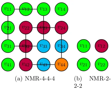
Figure 2.1. Solutions for various NMR problems

• its relation rel(c)⊆Dk ₌_D_×_{. . .}_×_D

| {z }

ktimes

where k =|scope(c)|, i.e. a subset of

possible k-tuples containing values from D.

A (partial) assignment A is a (partial) function A:V →D. A solution is an assignmentS, such that

∀c∈C,(S(vc1), . . . , S(vck))∈rel(c)

i.e. the values assigned to variables in scope(c) form a tuple in the constraint’s relation. In this case, I will say that constraintchas been satisfied2.

A binary CSP is a CSP consisting only of constraints with a scope of at most two variables.

I now introduce a running example to illustrate each of these concepts.

Example 2.1 (Non-monochromatic rectangle [Gas09]). The problem is to colour the cells of an m by n grid, using k colours and such that the cells at the corners of any rectangle may not be monochromatic, i.e. all take the same colours. I will call the instance with a m by n grid using k colours NMR-m-n-k. An example solution to NMR-4-4-4 is shown in Figure 2.1(a)3. Notice that a couple of rectangles are highlighted using lines on each side and are indeed non-monochromatic.

NMR-m-n-k can be encoded as a CSP (V, D, C) as follows:

2_{hence constraint}_satisfaction _problem

(29)

2.2. FUNDAMENTAL CSP ALGORITHMS 13

• A variable vij ∈ V for each cell (i, j) in the grid. Here the row i is indexed

first.

• A value valc ∈D for each colour c. For example,1 for blue and 2 for red. • For all choices of row indices i and j, and column indices k and l such that

i < j and k < l, a constraint cijkl ∈ C to ensure that the variables vik, vil, vjk and vjl are not all the same4.

Let cijkl =vik 6=vil∨vik 6=vjk∨vik 6=vjl then scope(cijkl) = (vik, vil, vjk, vjl) and

rel(c) =D4\ {(1,1,1,1),(2,2,2,2), . . . ,(k, k, k, k)}5_.

A = (v11,1),(v12,2),(v21,1),(v22,1) is a solution to NMR-2-2-2, shown in Figure

2.1(b).

2.2. Fundamental CSP algorithms

Constraint programming is the use of the CSP6 _{for solving practical problems.} Typi-cally this involves modelling a problem as a CSP, as above for NMR, and then using a

solver to find one or more solutions. However sometimes instead what is required is to satisfy the maximum number of constraints at once, optimise the solution according

to an optimisation function, etc. Solvers can becomplete orincomplete. Given enough time and memory, complete solvers guarantee to find a solution, if one exists, or to

report conclusively that none exists; incomplete solvers make no such guarantees. In

this thesis I will exclusively be concerned with complete solvers.

Complete algorithms for the CSP can be broadly categorised as eitherbacktracking search or dynamic programming solutions. Backtracking search algorithms predom-inate in practice because they have been found to be more memory efficient; more

flexible when it comes to solving related problems such as to find only the first or

optimal solution; and more time efficient in general [vB06].

Before introducing the algorithms I need to give some notations used throughout:

4_{called “not all equal” constraint in [}_BCR10_]

5_c

ijklcorrectly models “not all same” because it’s the negation of (vik=vil∧vik=vjk∧vik=vjl)

which is only true when the variables are all equal

(30)

Definitions 2.2. In search algorithms I will denote the domain of a variable v by initdom(v). Simply,D(v) = initdom(v). In many algorithms there exists a concept of the domain being narrowed, as values are ruled out, hence each variablev has its own domain dom(v), which is the subset of initdom(v) that has not already been ruled out at the current point in search.

If a constraint c is satisfied by all possible assignments to variables in scope(c) from their respective domains, cis said to be entailed.

I will first describe the classical backtracking (BT) search algorithm, before

pro-ceeding to describe the many available enhancements.

2.2.1. Chronological backtracking. Chronological backtracking (BT) is a sim-ple and effective base algorithm for solving CSPs. A BT solver for CSP will repeatedly

pick a variable by some means and then assign the variable one of its available values.

There are now 3 possible states:

(1) A solution has been found, in which case it is reported to the user; the solver

terminates7.

(2) One or more constraints are fully assigned but unsatisfied, the solver must

backtrack and try again.

(3) Neither of the above apply, the solver makes its next assignment.

Practically, the BT algorithm is implemented by pushing and popping the current

state of the variables. So when v is set to to value a, dom(v) = {a}, but after the solver backtracks beyond the point when this occurred, dom(v) will be restored to initdom(v). Pseudocode is given as Algorithm 18.

I will now present an example of the progress of BT search on NMR-2-2-2.

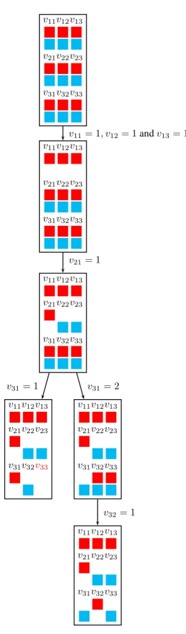
Example 2.2. The entirety of a search process can be depicted as a search tree. In a search tree the nodes are decision points, and the child subtrees represent the search in a recursive call. The search tree for NMR-2-2-2 with BT search is shown in Figure 2.2. There are few enough variables and values in NMR-2-2-2 that the state of the

7_{This is not essential, a solver could also proceed to look for more solutions.}

(31)

AlgorithmBT-SEARCH Search()

A1 if ∀v∈V,|dom(v)|= 1 A1.1 output solution

A1.2 exit

A2 choose a variable v to branch on s.t. |dom(v)|>1 A3 for val∈dom(v)

A3.1 push solver state A3.2 set dom(v) ={val}

A3.3 if ¬∃c∈C s.t.c is fully assigned and unsatisfied

A3.3.1 Search()

A3.4 pop solver state A3.5 return

Algorithm 1: Backtracking search

v₁₁v₁₂v₂₁v₂₂

1 2

v₁₁v₁₂v₂₁v₂₂

1 2

v₁₁= 1

v₁₁v₁₂v₂₁v₂₂

1 2

v₁₂= 1

v₁₁v₁₂v₂₁v₂₂

1 2

v₂₁= 1

v₁₁v₁₂v₂₁v₂₂

1 2

v₂₂= 1

v₁₁v₁₂v₂₁v₂₂

1 2

v₂₂= 2

Figure 2.2. Search tree for BT search on NMR-2-2-2

domain at each node can be depicted: in Figure 2.2 the variable name is shown above the colours represented by the values still remaining in its domain.

The first decision is to assign v11 to 1, i.e. blue, at A3.2 in Algorithm 1. The

(32)

third decision is to assign v21 to 1 and again no constraint is unsatified. The fourth

decision is the same: assignv22 to1, but this time the constraint is fully assigned and

unsatisfied. Hence the state is restored, and v22 is assigned to 2, i.e. red. Now the

recursive call happens and the solution is output at A1.1 and the solver can terminate.

Given enough time and space, BT search can solve any CSP. However several

improvements are available, and I will survey them briefly in the following sections.

2.2.2. Propagation. Propagation is when a constraint solver infers that one or more values in the domain of a variablev cannot possibly be part of a solution to the CSP. Those values are then removed from dom(v). In this way

• fewer incorrect assignments are available resulting in less fruitless search, and

• domain might be emptied allowing for immediate backtrack.

Various different levels of propagation are available (see [Bes06] for a general

survey), I will now describe several levels of consistency that will be relevant for this

thesis, with examples of the effect of each.

2.2.2.1. Generalised arc consistency. In short,generalised arc9consistency (GAC) on a constraint c ensures that given the current domains of the variables, no value remains that cannot be part of a complete assignment to all the variables in the scope

of the constraint.

Definition 2.1 (Generalised arc-consistency, adapted from [Bes06]). Given a CSP

(V, D, C), a constraint c∈C and a variable v ∈scope(c),

• A valid tuple is a tuple τ ∈rel(c) s.t. ∀i, τ[i]∈dom(scope(c)[i]).

• A valid tuple τ is a support for value val∈dom(x) iff ∃is.t. x=scope(c)[i] and val=τ[i].

• A value val ∈dom(v) is GAC with ciff there exists a valid tuple τ ∈ rel(c) s.t. τ[i] =valwhere i is the index of v in scope(c).

• A variable v is GAC with ciff ∀val∈dom(v), valis GAC with c. • The CSP (V, D, C) is GAC iff ∀c∈C,∀v ∈scope(c), v is GAC with c.

9_{“arc” refers to the constraint graph: consisting of a vertex for each variable and a hyper}

(33)

v₁₁v₁₂v₂₁v₂₂

(a) Before

v₁₁v₁₂v₂₁v₂₂

[image:33.595.242.363.77.132.2]

(b) After

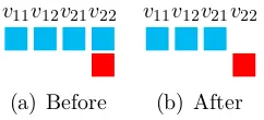
Figure 2.3. Before and after running GAC on the NMR-2-2-2 problem

• When the CSP (V, D, C) is GAC but ∃v ∈ V s.t. dom(v) = ∅, (V, D, C) is said to be arc inconsistent, or just inconsistent.

• On a binary CSP, GAC is called arc consistency (AC) but is otherwise the

same.

Various algorithms are available to enforce GAC on a CSP [Bes06] including AC3 [Mac77] and AC5 [HDT92]. Enforcing GAC means to take a set of domains

(one for each variable) and to output a set of domains with all GAC inconsistent

values removed, but no consistent values removed. Hence all the solutions of the

input domains are still present, but values may have been removed. AC3 and AC5

are variations on a simple theme: GAC can be enforced on the CSP by enforcing it

on constraints, variables and values until a fixed point is reached [Bes06].

I now give an illustration of these definitions on NMR-2-2-2 running example.

Example 2.3. Recall that NMR-2-2-2 has just one constraint that variables v11,v12, v21 and v22 must not all be the same. In Example 2.1 I said that this constraintchas

scope(c) = (v11, v12, v21, v22) and rel(c) ={1,2}4 _{\ {(1}_,₁_,₁_,₁₎_,₍₂_,₂_,₂_,_2)}_.

Suppose that GAC is enforced on NMR-2-2-2 when the domains are as shown in Figure 2.3(a). (1,1,1,2) is a valid tuple in rel(c) and hence 1 ∈ dom(v11), 1 ∈

dom(v12), 1∈ dom(v21) and 2 ∈ dom(v22) have been shown to be GAC for c. Hence

variablesv11, v12 and v21 are GAC forc because all their values are GAC.

It now remains to resolve whether 1∈ dom(v22) is GAC or not. Clearly no valid tuple includes this value because the remaining 3 variables are already assigned to blue then to set v22 to blue would mean all 4 were the same. Hence 1 ∈ dom(v22) is not

GAC.

(34)

In many constraint solvers GAC is maintained throughout search: it is enforced

before every decision is made. GAC has been shown to be a practically useful level

of consistency to enforce during BT search because:

• It is cheap to enforce. The worst case time complexity of enforcing GAC on

a binary CSP is O(ed2_{), where}_e ₌_|_C_| _and _d₌_|_D_| _{(using AC4 [MH86] or} AC2001 [BR01]).

• On many CSPs of practical interest enough values are removed by AC to

result in faster search overall [SF94].

Algorithm MAC-SEARCH Search()

A1 if ∀v∈V,|dom(v)|= 1 A1.1 output solution

A1.2 exit

A2 enforce GAC on allc∈C

A3 if ∃v∈V s.t. dom(v) =∅

A3.1 return

A4 choose a variable v to branch on s.t.|dom(v)|>1 A5 forval∈dom(v)

A5.1 push solver state A5.2 set dom(v) ={val}

A5.3 Search()

A5.4 pop solver state A6 return

Algorithm 2: Backtracking search maintaining arc-consistency

With GAC incorporated in the search process the search algorithm is as shown in

Algorithm 2. It is known as MAC, for maintaining arc consistency. The differences compared to Algorithm 1 (BT search) are as follows:

• GAC is enforced at line A2.

• If the CSP is GAC inconsistent, the solver backtracks (line A3.1).

• The recursive call at A5.3 is no longer conditional: the most recent

assign-ment cannot complete an incorrect assignassign-ment, otherwise GAC would have

removed the offending value10.

10_{Note, however, the entire CSP may now be GAC inconsistent and this is discovered in the}

(35)

GAC is the strongest possible level of domain consistency that can be enforced

by analysing constraints individually [Bes06].

2.2.2.2. Constraint propagators. In practice, consistency on a constraint cis usu-ally enforced by a constraint propagator forc. A constraint propagator takes as input a set of domains and returns domains where zero or more inconsistent values are

re-moved. Constraint propagators in an AC3 framework [Mac77] are told nothing about

how the domains have changed since they were last invoked. In more modern solvers,

propagators are told what has changed, hence they must maintain state if they want

to take full advantage. In Example 2.3 I gave an example of GAC propagation of the

“not all same” constraint which ensures its variables are not all equal, I now present

a GAC propagator for it.

Algorithm NOT-ALL-SAME-PROPAGATOR

BT<bool>allAssgsSame = true; int lastAssg;

BT<int>howManyAssgsSame = 0;

when vi ←a:

A1 if(!allAssgsSame) A1.1 return

A2 if(howManyAssgsSame == 0) A2.1 lastAssg = a;

A2.2 howManyAssgsSame = 1; A3 else if(lastAssg == a) A3.1 howManyAssgsSame++;

A4 else

A4.1 allAssgsSame = false; A4.2 return;

A5 if(howManyAssgsSame == arity - 1)

A5.1 prune a from variablevj that is not already set to a;

A5.2 allAssgsSame = false;

Algorithm 3: Propagator algorithm for “not all same” constraint

(36)

Now I describe the algorithm. At line A1, the algorithm stops immediately if the constraint is already satisfied, i.e. two assignments are known to be different. Between lines A2 and A4.1 the variables are updated to take into account the new assignment

vi ← a. If it’s the first assignment, they are initialised at A2. Otherwise at A3

when the assignment is to the same value as before howManyAssgsSame is advanced, or at A4 when it is different the constraint is now satisfied so allAssgsSame is set accordingly and the propagator stops (A4.2). Finally, the propagator checks if any propagation is necessary, which is the case when all but one variable is assigned the same.

This algorithm is amortized linear time down a branch of the search tree. Clearly

everything is constant time except for line A5.1. A5.1 takes time linear in the number

of variables, but the propagator must have run a linear number of times down the

current branch of the search tree in order to reach A5.1. Hence the time to check each

variable can be amortized against the earlier propagator invokations, to make each

invokation of the propagator amortized O(1) time and overallO(n) down a complete branch.

I will now complete the description of propagation by mentioning other, weaker

consistencies.

2.2.2.3. Consistencies weaker than GAC. Solvers are at liberty to enforce any level of consistency that works well in practice, provided only that an incorrect complete

assignment will lead to an immediate backtrack [SC06]. Consistency may be enforced

selectively on values based on their relative order; at other times an ad-hoc level of

consistency is chosen to perform a subset of available prunings easily.

I will call an algorithm that enforces consistency on a constraint c a propagation algorithm for c. As described above a propagation algorithm takes as input the variable domains, and outputs reduced domains.

For example, there is a consistency level calledbound(D) consistency (abbreviated to BC(D)) that guarantees only that the smallest and largest values belong to a

support, but not necessarily the ones in between. This is exploiting the numerical

(37)

v₁₁v₁₂v₂₁v₂₂

(a) BC(Z)

v₁₁v₁₂v₂₁v₂₂

(b) GAC

Figure 2.4. The NMR-2-2-3 problem in BC(D) and GAC consistencies

Definition 2.2(Bound(D) consistency (BC(D)), adapted from [Bes06]). For a CSP

(V, D, C),

• A variablev is BC(D) withciff min(dom(v)) is GAC withcand max(dom(v)) is GAC with c.

• The CSP (V, D, C) is BC(D) iff ∀c∈C, ∀v ∈scope(c), v is BC(D) with c. • When (V, D, C) is BC(D) but ∃v ∈ V s.t. dom(v) = ∅, (V, D, C) is said to

be bounds inconsistent.

BC(D) and related consistencies like BC(Z) and BC(R) are designed to find “low

hanging fruit”, that is inconsistent values that are easy to find, and are not intended

to be complete except coincidentally. They are very important in practical constraint

solvers because it is NP-hard to enforce GAC on some constraints [BHHW04]. Even

when not NP-hard, the cheapest GAC propagator may be a slow polynomial time

algorithm.

I will now illustrate the definition with the NMR running example.

Example 2.5. Recall that NMR-2-2-3 is the same as the NMR-2-2-2 example dis-cussed earlier, except it has 3 values (i.e. colours) for each variable (cell).

In Figure 2.4(a) the domains shown are BC(D) consistent. However they are not GAC, because the middle (green) value in dom(v22) is not part of a valid tuple. The

domains shown in Figure 2.4(b) are GAC.

2.2.2.4. Consistencies stronger than GAC. There are many other consistencies available for CSP that enforce a higher level of consistency than GAC. Since GAC is

the highest possible level of consistency that can be enforced on a single constraint,

these higher forms of consistency work by processing groups of constraints to find

disallowed assignments. I will briefly summarise a few of the most widely used

(38)

2.3. LEARNING CSP ALGORITHMS 22

Singleton arc consistency (SAC). Singleton arc consistency [DB97] is able to

iden-tify values that cannot appear in any solution.

Definition 2.3(Singleton arc consistency). Given a CSP (V, D, C), a variablev ∈V and a valuea∈dom(v): An assignmentv ←a is singleton arc consistent if and only if (V, D, C) is GAC when v ←a, i.e. dom(v) ={a}; otherwise v ←a is singleton arc inconsistent.

Any singleton arc inconsistent (SAI) assignment can be ruled out of future search,

i.e. if v ← a is SAI then remove a from dom(v). SAC is time consuming to enforce, requiring AC to be enforced for each variable and value pair. For this reason it is

typically enforced only at the root node but successful results have been shown for

both root node and maintaining SAC during search [LP96].

2.2.2.5. Other consistencies. Consistency and propagation is a central topic of constraint satisfaction. Hence I have given only a brief overview of consistencies,

especially where they are relevant to this thesis. More information can be found in

[Bes06].

2.3. Learning CSP algorithms

Having completed a brief survey of the components of a complete CSP solver, I will

now focus on the topic of this thesis: solvers that learn from experience. Previous

applications of learning in CSP search can be broadly classified as being either:

Backjumping: A normal solver will step back once after inconsistency is

dis-covered. Backjumping algorithms are sometimes able to make multiple steps after an inconsistency.

Learning new constraints: A normal solver retains the same set of

con-straints throughout search: those of the original problem. However it is

possible to achieve increased inference by augmenting the set.

Heuristics: The order in which variables and values are picked for

assign-ment can make a big difference: with an oracle a solution can always be

(39)

2.4. EXPLANATIONS 23

Some heuristics learn from experience to attempt to reduce search size, e.g.,

[BHLS04].

Historically, backjumping and learning new constraints (which I will call simply

learning from now on) have been closely related, because both rely on an analysis of the decisions and propagation that led to inconsistency, hence having done the

analysis for, say, constraint learning, it can make sense to also do backjumping.

So-calledexplanations, in some form, are a unifying concept in both constraint learning and backjumping and for this reason I will review explanations first. Techniques for

explanations are spread and often hidden throughout the history of learning.

For this reason I take a unconventional approach to reviewing this field. Often two

learning or backjumping algorithms can be viewed as identical or similar, except that

the explanation mechanism is varied. For this reason I first extract the explanation

algorithms from the mess of learning and backjumping algorithms. After that I

describe the essential techniques of backjumping and learning new constraints, based

on the understanding that often any explanation technique or a mixture of them can

be used.

2.4. Explanations

Explanations are a means for discoveringwhy a constraint solver makes an inference, why it cannot find a solution, etc. Such techniques have been used to allow a solver to

introspect and learn, but also for user feedback to assist with modelling and debugging

(e.g. [Jun01]). Explanations are dual to the common CSP concept of nogood, as I will describe shortly.

First I define the possible aspects of a solver’s current state that an explanation

pertains to:

Definition 2.4. If dom(v) = {a}for some variablev ∈V thenais said to beassigned to v; this is called an assignment and written v ← a. Similarly, if a /∈ dom(v) then a is said to be disassigned tov; this is called a disassignment and is written v ₈a. Collectively I will call them (dis-)assignments.

(40)

v₁₁v₁₂v₂₁v₂₂

×

Figure 2.5. Illustration of disassignment for NMR-2-2-3

Failures, assignments and disassignments are all solver events.

Explanations are intended to connect (dis-)assignments and failures with their

causes, which for present purposes will be other (dis-)assignments.

Definition 2.5. An s-explanation11 for a solver event e is a set of assignments that are sufficient for the solver to infereby some unspecified method. An explanation for eis minimal for propagator P if no event can be removed from it while still allowing a specific propagator P to infer e. An explanation is simply minimal if it is minimal for a GAC propagator. An explanation for event e is said to “label” the event.

A solver will usually make such an inference as a result of propagation, but the

definition leaves open any form of inference.

Example 2.6. Figure 2.5 shows an example of GAC propagation on NMR-2-2-3 from earlier Example 2.5. GAC has inferred that because v11, v12 and v21 are assigned to

2=green,v22 must be assigned to anything but green, in order to satisfy the constraint.

Hence the explanation for v22 82 is {v11 ←2, v12←2, v21←2}.

This type of explanation was used for most of the history of learning in CSP,

until g-learning12 was introduced by Katsirelos and Bacchus [Kat09] in a major

breakthrough that I will describe later. g-learning uses explanations that can be

composed of both assignments and disassignments:

Definition 2.6. Ag-explanation for a solver eventeis a set of (dis-)assignments that are sufficient for the solver to infere.

Clearly an s-explanation is a type of g-explanation. Inference is often based on

disassignments, not only assignments. For this reason g-explanations provide a closer

match for certain consistencies, e.g. GAC.

11_{the s stands for}_standard _{and the name is due to Katsirelos [}_Kat09_]

(41)

Example 2.7. Suppose that a CSP contains the constraint x = y. Suppose further thatx₈1. By GAC the solver can then infer that y₈1. The explanation fory₈1 is {x₈ 1}. This cannot be expressed by an s-explanation involving only variables x

and y, because there has been no suitable assignment to x (indeed there has been no assignment to x at all).

Explanations are not necessarily unique, there may be several minimal

explana-tions for an event. This fact is exploited by at least one learning algorithm [SV94].

It is important to emphasise an essential property of explanations when they are

used in practice (see [NOT06] for an equivalent property used in SMT solvers).

Suppose explanation {d1, . . . , dk} labels pruningv 8a:

Property 2.1. All ofd1, . . . , dk must first occur beforev 8a.

Remark 2.1. Ensures that causes must precede effects13. This simply takes into

account that there may exist multiple possible explanations, but I am presently

in-terested in the unique explanation that was actually used to do an inference.

I will now proceed to describe schemes for generating explanations and their

char-acteristics and merits.

2.4.1. Generic techniques. Suppose that all decisions made by the solver are

assignments, then {v ← a : v ← a is a decision, v ← a 6= e} is an s-explanation for any event e, i.e. the explanation for e is all the decision assignments excluding the event itself (if necessary). This is a rather pointless explanation which usually says

little about the intuitive reason fore. It works because if all the decision assignments were repeated, assuming the same level of propagation was enforced, the same event

must eventually be obtained.

As shown in [Kat09], such an explanation can be improved using a generic

min-imisation technique called quickXplain [Jun01]. quickXplain may need to enforce

consistency on a set of propagatorsO(k2) times wherek is the size of the explanation to begin with. Katsirelos claims that this overhead is too large for minimisation to

13_{avoiding cycles in the g-learning implication graph [}_{MSS96, Kat09}_{] to be defined later in}

(42)

be practically worthwhile [Kat09]. Also, as I describe in the following sections, often

a minimal explanation can be computed directly and efficiently.

Another generic technique is used in Dechter’s graph-based backjumping (GBJ)

(Section 2.5.4) andgraph-based shallow learning [Dec90]. It exploits the observation that an explanation for a (dis-)assignment to variablev can only include assignments to variables connected to v through the scope of one or more constraints. All such assignments are included in the explanation, hence the result is a subset of that

obtained by the above generic scheme for s-explanations. The explanations are not

necessarily minimal, but are easy to compute. In [Dec90] such an explanation for an

assignment is called its graph-based conf-set.

Dechter [Dec90] also suggests how to explain a failure due to variablef14having no remaining consistent values: Start with the partial assignment at the point in

search where the failure occurs. Remove any assignment from A that is consistent with all values in the failed var f; or, alternatively, ensure that A contains only assignments that are in conflict with at least one value inf. Formally, v ←acan be removed fromA if constraint c with scope(c) = (v, f)15 is such that ∀val ∈dom(f), (a, val) ∈ rel(c), i.e. v ← a does not conflict with any value of f. This technique is used infull shallow learning in conjunction with forward checking [HE79].

2.4.2. Generic techniques based on propagation. Since many solver events

are derived by propagators, explanations for propagation should be available. As

shown in Example 2.7 the reasoning behind propagation routinely cannot be

di-rectly expressed as an s-explanation and it was not until Katsirelos and Bacchus’

work on g-learning [KB03] that more expressive g-explanations were used for this

purpose. Katsirelos gave a generic scheme for explaining propagators in his thesis

[Kat09]: Suppose that event vk ← a (or vk 8 a) is forced by the propagator for constraint c which has scope(c) = (v1, . . . , vk). The propagator can only have used (dis-)assignments to variables in the set {v1, . . . , vk−1} in its reasoning. Hence the explanation is the set of all assignments (if possible) and disassignments to those

variables. It should be clear that some of these (dis-)assignments had no effect on the

14_called _f _{because it caused the failure}

(43)

propagation in question and so the explanation is imprecise. I will illustrate with an

example:

Example 2.8. Suppose that a CSP contains the constraint x = y. Suppose further that x ₈ 1 and x ₈ 2. The propagator for x = y is able to infer that y ₈ 1 and an explanation of {x ₈ 1, x ₈ 2} would be produced by the above generic scheme. However, as shown in Example 2.7, just{x₈1} is a valid and shorter explanation.

These explanations can again be improved by a generic minimisation routine like

quickXplain.

Prosser’s CBJ in its various forms (CBJ, FC-CBJ, MAC-CBJ) can also be viewed

as explanation-producing algorithms [Pro93b, Pro95]. Indeed, they were used as

such in [FD94]. I will revisit these algorithms later when I review backjumping

(Sec-tion 2.5) but for now describe how MAC-CBJ produces explana(Sec-tions for assignments

and failures16.

Each variable v has a conflict set CS(v) , which is the set of variables whose assignments have directly or indirectly caused the removal of a member of dom(v):

• When a variable v is assigned in a decision v ←a,CS(v) is set to {v}. This reflects that the assignment itself caused the removal of several values.

• When a propagator for constraint c with scope(c) = (v1, . . . , vk) causes an (dis-)assignment to variablevj,CS(vj) is assigned to

Sk,i6=j

i=1 CS(vi). The new conflict set incorporates the reasons why all the variables in scope(c) have the values they do, and hence why the propagation happened.

Now the explanation for a failure in variablev (if v has failed) or an assignment tov (if it is assigned) is just the set of assignments variables inCS(v). Such explanations may not be minimal, but are more precise than GBJ or the other generic schemes so

far described.

I now proceed to describe explanation techniques that are even more precise,

because they take into account exactly why propagators behave as they do.

(44)

[OSC07] [Kat09] [Sub08] [Vil05] [RJL03] [SFSW09] [GJR04] Product Y(es)

Inequality Y Y

Lex≤ Y

Alldiff Y Y

GCC Y

Roots+range Y

Table Y

BDD Y

Scheduling Y Y

Stretch Y

Flow Y

Table 2.1. Global constraints and the papers in which they have been

given invasive explanations

2.4.3. Specialised techniques based on propagation. The next level of

ex-planation technology is to generate exex-planations for (dis-)assignments with full

knowl-edge of the propagation that occurred, in other words, inside the propagator. This

affords the opportunity to produce explanations with no superfluous (dis-)assignments

and to directly encapsulate propagation reasoning.

This general approach has been used before with:

• Propagators enforcing GAC [Kat09, OSC07], bound consistencies [OSC07,

Kat09] and specialised consistencies [Vil05].

• Many different constraints, see Table 2.1.

• Different types of explanation including g- and s-explanations.

The essence of the approach is that the propagation algorithm is adapted to

not only do disassignments, but also to store an explanation for each disassignment

[JDB00a]. I will call these invasive explanations. Invasive explanations:

• need not be minimal (e.g. Nogood-GAC-Schema-Allowed-log-approx from

[Kat09]);

• may be computed at the time of propagation (usually) or retrospectively (e.g.

[Vil05, NO05]); and

• may be either g-explanations [Kat09], s-explanations [Sub08, RJL03] or

(45)

Advances in invasive explanations will form a major part of this thesis, however

since many of the algorithms of Table 2.1 will be revisited in Section 3.5 in detail I

will not describe them here. However to provide an introduction I will now illustrate

the technique by continuing the NMR running example.

Algorithm NOT-ALL-SAME-EXPLAINING-PROPAGATOR

... ...

A5 if(howManyAssgsSame == arity - 1)

A5.1 remove a from dom(vj) where remaining variable isvj;

A5.2 store explanation {vi←a:vi ∈V, i6=j} forvj 8a

A5.3 allAssgsSame = false;

Algorithm 4: Explaining propagator algorithm for “not all same” constraint

Example 2.9. Example 2.4 contains a propagation algorithm for the “not all same” constraint. An excerpt is reproduced as Algorithm 4. At line A5.2 the explanation is stored.

This intrusive explanation code is typical: when the propagator removes a value

it must also store an explanation. In this case, the amortized complexity of the

propagator is unchanged. The explanation is minimal.

2.4.4. Nogoods. The concept of a nogood has been common in CSP learning literature (e.g. [Kat09, Dec03, Dec90] and others). Nogoods are closely related to

explanations:

Definitions 2.3 (Nogood). A g-nogood for (V, D, C) is a set of (dis-)assignments that cannot all be true in any solution.

An s-nogood is a g-nogood containing only disassignments.

I will now make precise the relationship between explanations and nogoods.

Lemma 2.1. E is an g-explanation for v ←a iff E∪ {v ₈a} is a g-nogood.

Proof. (⇒) If everything inE is true, then the propagation logically determines

that v ← a must hold. Hence v ₈a must not hold along with E and E ∪ {v ₈a} is a g-nogood.

(46)

2.5. BACKJUMPING 30

exists a level of inference, for example unit propagation, which would infer{v ←a}

using onlyE, hence it is an explanation for v ←a.

I now continue to a review of backjumping, which is conceptually easier than

constraint learning, and arguably played a bigger part in the early history of CSP

solvers.

2.5. Backjumping

Before describing several concrete backjumping algorithms I will illustrate the

tech-nique by an example.

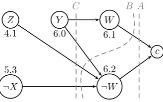
Example 2.10. Consider the problem NMR-2-3-2, but with the additional constraint

v13 = v23. Suppose chronological backtracking (BT) plus an unspecified type of

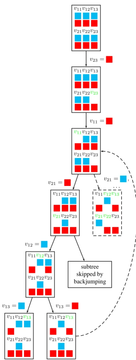
back-jumping is used for search. A whole search tree is shown in Figure 2.6. The sequence of decisions and inferences is as follows:

(1) Set v23= 2. (2) Set v11= 2. (3) Set v21= 2. (4) Set v12= 1.

(5) Set v13= 1. The constraint v13 =v23 is failed. The solver backtracks.

(6) Set v13 = 2. The “not all equal” constraint with scope (v11, v13, v21, v23) is

failed, because all cells are red. The most recent choice point with options still remaining is for variable v12, but changing this option does not help at all:

it had no influence on the failure and the solver still cannot give a consistent assignment tov13. Hence it is preferable to backjumpto reassign v21 instead. (7) Eventually a solution will be found after the assignment v21= 1.

At step 6, if the solver were to instead try a different choice forv12it would proceed to fail for the same reason. In BT search this is called thrashing. Generally, search algorithms like this which skip parts of the search tree by making multiple steps are

calledbackjumping algorithms. Such algorithms avoid thrashing, because they avoid some making some assignments which are certain to fail (however thrashing is still