Distribution based fuzzy clustering of electrical resistivity tomography images for interface detection

Geophysical Journal International

Geophys. J. Int.(2014)197,310–321 doi: 10.1093/gji/ggu006

Advance Access publication 2014 February 11

GJI

M

arine

g

eosciences

and

a

pplied

g

eophysics

Distribution-based fuzzy clustering of electrical resistivity

tomography images for interface detection

W.O.C. Ward,

P.B. Wilkinson,

J.E. Chambers,

L.S. Oxby

and L. Bai

2_{British Geological Survey, Nottingham NG12 5GG, UK}

Accepted 2014 January 8. Received 2014 January 7; in original form 2013 June 21

S U M M A R Y

A novel method for the effective identification of bedrock subsurface elevation from electrical resistivity tomography images is described. Identifying subsurface boundaries in the topo-graphic data can be difficult due to smoothness constraints used in inversion, so a statistical population-based approach is used that extends previous work in calculating isoresistivity sur-faces. The analysis framework involves a procedure for guiding a clustering approach based

on the fuzzyc-means algorithm. An approximation of resistivity distributions, found using

kernel density estimation, was utilized as a means of guiding the cluster centroids used to classify data. A fuzzy method was chosen over hard clustering due to uncertainty in hard edges in the topography data, and a measure of clustering uncertainty was identified based on the reciprocal of cluster membership. The algorithm was validated using a direct comparison of known observed bedrock depths at two 3-D survey sites, using real-time GPS information of exposed bedrock by quarrying on one site, and borehole logs at the other. Results show similarly accurate detection as a leading isosurface estimation method, and the proposed algo-rithm requires significantly less user input and prior site knowledge. Furthermore, the method is effectively dimension-independent and will scale to data of increased spatial dimensions without a significant effect on the runtime. A discussion on the results by automated versus supervised analysis is also presented.

Key words: Image processing; Neural networks, fuzzy logic; Tomography.

1 I N T R O D U C T I O N

Intrusive investigation, especially drilling, is the most signifi-cant and common method by which to analyse shallow soft-rock aggregate mineral resources in unconsolidated superficial geolog-ical deposits (e.g. sand and gravel). A complementary method, involving minimal intrusion, is electrical resistivity tomography (ERT), which has been demonstrated as a viable means of min-eral deposit characterisation. Known benefits of ERT imaging over direct intrusion include the provision of spatial information and rapid non-invasive survey coverage. Although ERT imaging of the subsurface is not yet routinely used for soft-rock aggregate explo-ration, research has been undertaken in recent years to develop ERT for this application (e.g. Hirschet al.2008; Hickinet al.2009; Hsu

et al. 2010; Chamberset al.2012,2013; Lokeet al.2013). The purpose of such studies is to provide the evidence base needed to validate ERT for this application, and to establish a good practice framework covering survey design, data processing and interpreta-tion, and the integrated use of ERT (e.g. B¨ohmet al.2013) alongside conventional intrusive techniques (i.e. drilling and trial pitting).

Accurate delineation of subsurface boundaries or edges is essential to achieve reliable estimates of overburden volumes and

minerals reserves. Common image processing approaches to edge detection typically involve gradients in the image. Such attempts on ERT images are detailed in Hsuet al.(2010) and Chamberset al.

(2012,2013). Problems occur, however, if the steepest gradients in the image do not coincide with the locations of the mineral inter-faces, which can occur due to the nature of smoothness-constrained inversion and the fundamental lack of resolution at depth, even when the true interface is sharp. However, in certain cases where deposits are relatively homogeneous, resistivity isosurfaces can be used instead to identify interfaces (Chamberset al.2013).

In this study, the aim was to develop a reliable method for the analysis of 3-D ERT images generated using standard 3-D ERT survey and inversion approaches to delineate mineral volumes and thereby estimate yields. Due to the gradational transitions in the ERT images, a fuzzy algorithm was chosen. It involves edge detec-tion based on a machine learning approach, incorporating clustering methods guided by exploiting the probability density properties of the resistivity image. A framework was developed to automatically determine the density function. It was found that a probability den-sity function (pdf) provided a suitable means of guiding cluster initialization that both increased accuracy and significantly reduced the runtime. The accuracy of the method was improved by choosing

310 _{distributed under the terms of the Creative Commons Attribution License (}CThe Authors 2014. Published by Oxford University Press on behalf of The Royal Astronomical Society. This is an Open Access article_{http://creativecommons.org/licenses/by/3.0/), which permits} unrestricted reuse, distribution, and reproduction in any medium, provided the original work is properly cited.

by guest on October 19, 2016

http://gji.oxfordjournals.org/

Figure 1.Density distribution by histogram and KDE approximation on the Norton Disney site showing similarities in structures displayed. Control parameters were 50 equal width histogram bins and kernel bandwidthbw=0.05.

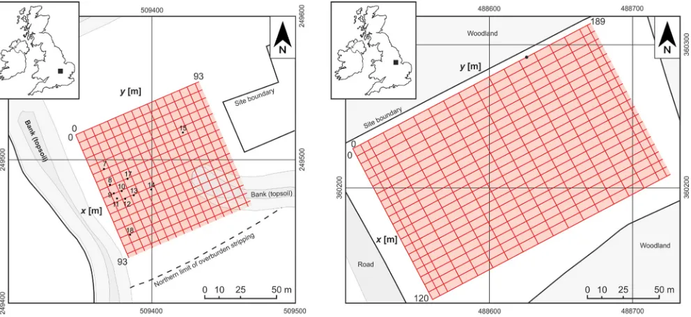
Figure 2.Three-dimensional ERT survey designs for the Willington (left) and Norton Disney (right) sites, showing survey areas (red shading), lines (red lines) and borehole positions (black dots).

the number of clusters to match the expected number of formations under investigation.

2 T E C H N I Q U E S / M E T H O D O L O G Y

2.1 Kernel density estimation (KDE)

The application of ERT can provide fully 3-D volumetric models of subsurface resistivity distributions. Features of contrasting resis-tivity can be located and characterized using KDE, a method for estimating the pdf of random variables. KDE is similar to creating a histogram to represent the distribution of data, except that it sums a symmetric weighting function, called a kernel, applied to each point in the data, rather than assigning each point to an interval. This provides large responses at areas of high frequency, that is, common values in the data (Botevet al.2010). An example of this is shown inFig. 1, which demonstrates the similarities in shape between KDE and histogram estimation.

Given N sample points of a random variable X =

{x1,x2, . . . ,xN} of an unknown continuous pdf,f, the KDE of f

atx∈R, ˆfσ(x), is defined by

ˆ

f_σ(x)= 1

N

N

i=1

K_σ(x−xi),

whereKσ(·) is the kernel function andσ is the bandwidth, a

pre-defined smoothing parameter ofK(Lanh1990). Like the choice

of interval size in a histogram, the bandwidth is an important con-sideration that strongly influences the density estimate. A small bandwidth will give a distribution containing many small peaks, whereas choosing a large bandwidth will give wide responses and return a very smooth curve with few, wider variations.

The kernel used on the data in this research is the Gaussian function,

K_σ(x)=φ(x;σ)= 1 σ√2πe

−x2

2σ2,

by guest on October 19, 2016

http://gji.oxfordjournals.org/

312 W.O.C. Wardet al.

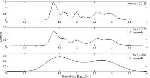
Figure 3.Probability density functions of Norton Disney ERT data. The top is the pdf result using kernel density estimation with automated bandwidth detection (Sheather & Jones1991). The detected bandwidth for this isbw=0.0126. The middle plot shows smoothing applied to the top plot, with resulting peaks identified by red circles. The bottom shows KDE applied with a wider, manually selected bandwidth ofbw=0.3, showing two detected peaks representing cluster centroids.

where each sample pointxirepresents the mean of the kernel

distri-bution inK_σ(x−xi) andσis the kernel bandwidth.

There exist multiple methods for selection and analysis of band-width suitability (Sheather & Jones1991; Botevet al.2010), and an automated approach is considered in this research to contrast with manual selection is the improved Sheather–Jones method proposed

by Botevet al.(2010). This method involves a completely

data-driven iterative scheme based on sample variance: for a number of estimated bandwidths, functionals are calculated, each being used to approximate the next until an optimal bandwidth for the data is found. An optimal bandwidth is one which minimizes the mean square error between the estimation and the true density function. This is approximated as a solution to a differential equation based on the assumed asymptotic behaviour of the error (Rosenblatt1956).

2.2 Fuzzy clustering

The process of clustering data is the task of grouping a set of ob-jects within a data set in such a way that obob-jects of the same group are more similar to each other in a particular way than those in other groups. It has many applications, such as pattern recognition,

image analysis and machine learning (Estivill-Castro 2002).

Clustering techniques may be classified in terms of how they han-dle data and rate object similarities: the major types are hierar-chal; distribution-based; density-based and centroid-based cluster-ing. Because of the nature of data in this study, the method used belongs to the centroid-based clustering family. It is largely based on fuzzyc-means (FCM) clustering, which, in turn, takes its theory

from the commonly usedk-means clustering method (MacQueen

1967). Thek-means algorithm is an unsupervised method for

sta-tistically classifying data. For some specified number of clusters, the method assigns each datum based on the minimized distance

to the cluster’s geometric centroid. The clusters are updated based on the new members, new centroids are found and the points are reclassified. This continues until the method reaches convergence between iterations.

An alternative to assigning data to specific clusters with an absolute in or out value is for a fuzzy subset to represent the point in relation to each cluster. This set assigns a fuzzy value to each datum for each cluster, similar to a probability value, based on the likeli-hood of membership of the datum into that cluster. FCM clustering makes use of this concept, assigning fuzzy membership values based on some measure of the distances of the data from the cluster cen-troids (Cannonet al.1986). Forndata pointsX= {x1,x2, . . . ,xn}

andcclusters, a fuzzy partition of a data set can be described by ac×nreal matrixU. The entries ofUmust satisfy the follow-ing conditions, withu:X →[0,1] being a function to assign each

x∈Xits grade of membership to each cluster in the fuzzy set: 1.Ui = {ui(x1),ui(x2), . . . ,ui(xn)}is theith fuzzy subset ofX,

that is, theith membership function. 2.Uj _{= {u}

1(xj),u2(xj), . . . ,uc(xj)}are the values of thec

mem-bership values of thejth data point inX.

3._iui(xk)=1,∀k, that is, the sum of membership values for

a data point is equal to 1.

4. 0<_kui(xk)<n,∀i, that is, no fuzzy subset is empty or

contains all ofX.

A fuzzy partitionU(0)_{is randomly generated based on the above}

criteria, and this is used to initialise the FCM method. A step functionb=0,1,2, . . . is initialized and theccluster centroids, contained in the set v, ofU(b) _{are calculated using the weighted}

membership function for theith cluster centroid:

νi = n

k=1[ui(xk)m·xk] n

k=1ui(xk)m

.

by guest on October 19, 2016

http://gji.oxfordjournals.org/

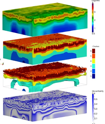
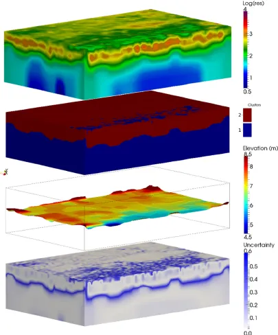
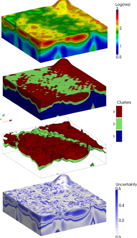
Figure 4. ERT model of Norton Disney site (top) with 6-clustering guided with a smoothed pdf estimated using automated bandwidthbw=0.0126, and calculated interfaces of deposits. The bottom model shows the uncertainty of the clustering as the reciprocal of fuzzy membership used to assign clusters.

An updated fuzzy subsetU(b+1) _{can then be found using the}

weighting cluster assignment operation:

ui(xk)= ⎡ ⎣c

j=1

di k

dj k 2

m−1 ⎤ ⎦

−1

∀i∈ {1, . . . ,c},∀k∈ {1, . . . ,n}.

The distance function, di k = ||xk−νi||, is based on some

arbitrary inner product norm, andm∈[1,∞) is a fixed weighting exponent. The FCM algorithm uses an iterative optimization to

approach minima of U, and thus requires convergence less than

some chosen error term. This can take significant computational effort to cluster sufficiently complex data, and due to the random nature of the initial step, may take varying lengths to reach convergence that may also be different in repeat applications due

to the dependence onU(0)_{. It is typical to bound the number of}

iterations such thatb<bmaxand if convergence is not reached, the

final clustering partition is taken to beU=U(bmax)_{. Furthermore,}

the method needs to be initialized with some value for the number of clusters,c.

For the purpose of all analysis in this paper, the weighting expo-nentm=2, and the distance norm used in cluster assignment is the Euclidean norm,||x|| =x2_i.

2.3 Guided fuzzy clustering

The random element of the application of FCM to a data set leads to an analysis tool that does not provide identical results upon repeat applications and, in cases of some randomly generated choices of

by guest on October 19, 2016

http://gji.oxfordjournals.org/

314 W.O.C. Wardet al.

Figure 5.ERT model of Norton Disney site (top) with 2-clustering guided with a pdf estimated using the manually selected bandwidthbw=0.30 (second). The interface between the two clusters is taken to be the bedrock surface and an elevation map is shown. The bottom model shows the uncertainty of the clustering as the reciprocal of fuzzy membership used to assign clusters.

U(0)_{, will not give adequate clustering detail, whereas a different}

choice ofU(0)_{would under the same conditions. In order to remove}

this inconsistency in cluster membership, a method to guide the fuzzy clustering is introduced. The method also identifies a desirable cluster number as part of the generation ofU(0)_.

For the data setXrepresenting the random variable (in this study, resistivity values at each datum), the fuzzy subsetU(0) _ofXmay

be calculated using the weighted cluster assignment of FCM on some pre-defined set of cluster centroids,ν(−1)_{. Here, the centroids}

are pre-calculated by first approximating the density distribution of the data set. Applying the KDE method to the data and finding an approximation ˆf(x) provides a statistically grounded analysis of the data set. Each peak in the pdf shows an estimation of individual

populations in the data. Using the Gaussian kernel in the calculation

of ˆf means that the location of the maximum of each data peak

is approximately the mean of its corresponding data population. Therefore, the number of peaks can be assumed to represent the appropriate number of clusters required to group the data. Each cluster has a centroid equal to the value of its population density maxima, andν(−1) _{is calculated such thatν= {x¯}

i,i=1,2, . . .},

wherec= |ν|is the number of population means, ¯xi, in the setv.

Using this statistical approach to cluster initialisation removes the necessity of iterative optimization. Assuming that the bandwidth,σ, in the kernelK_σis appropriate for the data set, the peaks themselves represent adequate finalized centroids for clusters. This means that using this distribution-guided fuzzy clustering,U≡U(0)_{such that}

by guest on October 19, 2016

http://gji.oxfordjournals.org/

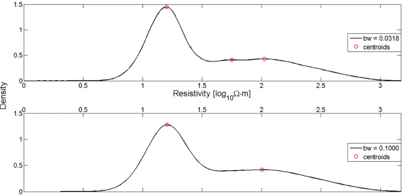
Figure 6. Probability density functions of Willington ERT data, using kernel density estimation of automated (top) and manually selected bandwidths. The detected population peaks that correspond to cluster centroids are identified by red circles. The automatically detected bandwidth was calculated as

bw=0.0318, whilebw=0.10 was chosen to approximate only two populations.

Urepresents the final fuzzy partition containing membership values forX.

To obtain a finalc-clustering of the data set, at each data pointxi,

the maximum membership value inUis taken as the absolute

mem-bership. The additional fuzzy information can be used to classify uncertainty in the final cluster model.

2.4 Geological population segmentation

While the most common and popular approaches to edge detec-tion use gradient informadetec-tion in multiple spatial direcdetec-tions to iden-tify interfaces between objects in the model or image (Chambers

et al. 2012), this approach may be limited by the gradational nature of smoothness constrained ERT images and the fundamental decrease in resolution with increasing distance from the electrodes

(Wilkinsonet al.2012). While most approaches have been tested

on 2-D ERT data (Sass2007; Hsuet al.2010), some extensions

of existing methods have been used on 3-D data sets (Chambers

et al.2012,2013). The method proposed here ignores the spatial properties of the resistivity image and analyses the data solely on the statistical distribution of the resistivities. Using some mapping function,χ:R3_{→R, that converts 3-D coordinate structural data}

to an ordered 1-D set of resistivity values, distribution-guided fuzzy clustering can be applied. The resulting ordered fuzzy membership set is then used to assign each resistivity values to the cluster for which it has maximum membership. Applying the inverse mapping χ−1_:R→R3_{, to the 1-D ordered cluster detail vector gives a 3-D}

clustered set, corresponding to the original resistivity image. The interfaces between the clusters are then assumed to represent the geological boundaries.

3 S T U D Y S I T E S

3.1 Willington

The first site used in this study is located in the valley of the Great Ouse, around 4 km east of Bedford, UK, near the village of Will-ington (Fig. 2a). The Great Ouse is an important part of the Wash

fluvial network, preserving a record of late Quaternary uplift and climate variation. It also contains records of Palaeolithic human activity.

In terms of geology, the site is composed of Quaternary alluvium and river terrace sand and gravel overlying Oxford Clay

forma-tion bedrock (Jurassic—Borehamet al.2010). The Oxford Clay

bedrock consists of the Peterborough member, a brownish grey, fissile mudstone. It crops out to both the southeast and northwest of the survey area and has an approximate thickness of 20 m, partly exposed by extractive activities in the river valley. The river terrace deposits here are of Ouse Valley formation, likely to have been formed by braided rivers under periglacial conditions during dif-ferent Quaternary cold stages (Rogersonet al.1992; Greenet al.

1996; Bridgland2006). There are three principle deposits observed

in the area (Horton1970; Barronet al.2010; Borehamet al.2010): the first is approximately 3 m thick, overlies Felmersham member and has a surface that is 0.6–2 m above the floodplain. The next terrace, with a surface 2–7 m above the floodplain, overlies Stoke Goldington member. The third terrace overlies Biddenham member, and is up to 7 m thick, its surface lying between 11 and 13 m above the floodplain. Sands and gravel of these three terraces display a similar composition, and are composed of a planar-bedded brown-ish yellow sand and gravel, which is mainly made up of flint and limestone.

The present day floodplain at the Willington site is covered by a brown clay and silt alluvium, which is up to 4 m thick and overlies Ouse Valley formation. In places, this may occupy channels that were cut in the Felmersham member by meandering rivers under temperate climate condition (Barronet al.2010).

There has been extensive removal and reworking of superficial deposits that have occurred from mineral extraction in this area, particularly quarrying of sand and gravel from river terrace deposits. In many places, there has been exposure of bedrock as a result of the removal of sand and gravel.

The study site is situated on terrace deposits of undifferentiated Felmersham and Stoke Goldington members, overlying Oxford Clay bedrock. The terrace deposits are the focus of long-standing sand and gravel operations, and at the time of study, the topsoil was stripped and banked, exposing alluvium at surface.

by guest on October 19, 2016

http://gji.oxfordjournals.org/

316 W.O.C. Wardet al.

Figure 7. ERT model of Willington site (top) with 3-clustering guided with a smoothed pdf estimated using automated bandwidthbw=0.0318, and calculated interfaces of deposits. The bottom model shows the uncertainty of the clustering as the reciprocal of fuzzy membership used to assign clusters.

This area was selected mainly because of the availability of good subsurface data in the form of borehole logs, which can be used to interpret and calibrate the geophysical results. Deposits are unsat-urated due to dewatering in mineral working immediately south of the study site.

3.2 Norton Disney

The second site detailed is a sand and gravel quarry near Norton Disney, Lincolnshire, approximately 10 km northeast of Newark and the River Trent (Fig. 2b). At the time of the survey, the site was a grassed field bounded by woodland, and the land immediately surrounding the area had been worked for sand and gravel for many years. After the ERT survey was completed, the site was quarried revealing much of the bedrock across the survey area.

The geology of the Norton Disney site consists of Quater-nary river terrace deposits of Balderton Sand and Gravel Member and a thin layer of topsoil, overlying flat lying Lower Lias mud-stone bedrock (Jurassic—Berridgeet al.1999). The Lias Group is

Figure 8.ERT model of Willington site (top) with 2-clustering guided with a pdf estimated using the manually selected bandwidthbw=0.10 (second). The interface between the two clusters is taken to be the bedrock surface and an elevation map is shown. The bottom model shows the uncertainty of the clustering as the reciprocal of fuzzy membership used to assign clusters.

composed mainly of grey shaly mudstone, with minor limestone, sandstone and ironstone beds. The site itself lies in the Scunthorpe Mudstone Formation, in the lower Lias Group, the formation of which is characterized by grey, variably calcareous, silty mud-stone with numerous thin limemud-stones. These limemud-stones are typi-cally around 0.1–0.3 m thick and can be well cemented and laterally persistent.

The Balderton Sand and Gravel Member is an early River Trent deposit, with a surface level around 14 to 15 m above Ordnance Datum at the Norton Disney site. The deposit at the site has a thickness of between 7.8 and 9.8 m, and is brown and yellow-brown according to borehole logs. The bulk of the deposit is slightly silty fine to coarse grained gravelly to very gravelly sand, and very sandy gravel. The deposit has poorly bedded gravels at the base, with sandier gravels further up and brown to orange-brown sandy, gravelly soil at the surface.

Borehole data were available for this site, the most recent being from 2005, including holes drilled close to the ERT survey area. Records for water levels close to the site indicate that they were

by guest on October 19, 2016

http://gji.oxfordjournals.org/

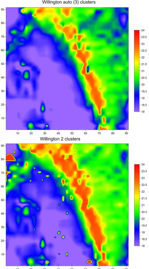
Figure 9.Elevation maps of detected bedrock for Willington site using three clusters (top) and two clusters.

likely to have been approximately 4 m below ground level. After quarrying, a real-time kinematic GPS survey of the exposed bedrock

surface was conducted (Chamberset al.2013) to provide ground

truth with which to compare the results of ERT interface detection.

3.3 ERT data collection & inversion

Methodological descriptions of ERT deployment and image gener-ation at the study sites are given by Chamberset al.(2012,2013), so only brief descriptions of data collection and inversion are provided here.

For the Willington site, the survey was carried out in an area of

93 m×93 m, using 16 survey lines positioned at 6 m intervals

in both thex-and y-directions. Data were collected using dipole– dipole configurations with dipole lengthsa=3 and 6 m and sep-arations of 1ato 8a. For the Norton Disney site, the survey area dimensions were 120 m×189 m, using 21 lines at 6 m intervals in thex-direction and 16 lines at 12 m intervals iny- direction. Dipole

a single-line direction in the ERT inversion is minimized by the use of orthogonal lines (Gharibi & Bentley2005). Dipole–dipole arrays were used as they provide a relatively high level of resolution, and can be efficiently acquired with multichannel ERT instruments in both normal and reciprocal configurations (Dahlin & Zhou2004). The reciprocal configuration is found by exchanging current and potential dipoles, and gives the same result as the normal configu-ration in the absence of non-linear effects. The difference between the normal and reciprocal configuration can therefore be used to assess random and certain systematic sources of error (Wilkinson

et al.2012). Here, the reciprocal error is defined as percentage stan-dard error in the mean of the forward and reciprocal measurements. The data sets from the Willington and Norton Disney sites com-prised 11 270 and 46 196 pairs of normal and reciprocal measure-ments, respectively. Pairs with reciprocal errors greater than 5 per cent were removed from the data set. This data removal accounted for only 2 per cent of the Willington data but approximately 13 per cent of data were removed for the Norton Disney site. This relatively high level of reciprocal errors can be accounted for by the presence of high contact resistances recorded during the field survey, which limits the current that can injected into the subsurface (Chambers

et al.2013).

Field data were inverted using a 3-D regularized least-squares optimization algorithm (Loke & Barker1996) and the resulting forward problem was solved using the finite-element method. After inversion, the resulting model for the Willington site contained

10 571 model cells of dimension 31×31×11 (x×y×z), and

20 160 cells for Norton Disney, with shape dimensions 40×63×8. For the Willington data, the model was produced using an L2-norm constraint. This was chosen because the site has significant gradational lithological variations that are observed in drift deposits and undulating topography of bedrock. In contrast, an L1-norm constraint was found desirable for the Norton Disney site. This method of inversion minimizes the sum of absolute values of the changes in model resistivity (Lokeet al.2003), leading to sharper changes within the inverted model. This was suitable since the Norton Disney deposit is dominated by sharp boundaries in the interface of sand and gravel and more conductive clay bedrock (Chamberset al.2013).

4 R E S U L T S

A comparison of results at the Norton Disney site with its ground truth was undertaken. After the ERT survey, the site was excavated and bedrock details for a large proportion of the site are known. Using the guided clustering method, two levels of cluster detail were identified: the first used the pdf from an approximation with automatically detected bandwidth (Botevet al.2010) that were then smoothed by a moving average method to remove superficial local maxima. This identified six populations which can be seen in the pdf inFig. 3. However, this did not reflect the broad geological divisions observed at the site (i.e. river terrace sands and gravels overlying mudstone bedrock) and so a manually selected bandwidth was also used that gave two distinct populations. This was chosen by reviewing the generated density function and adjusting the band-width accordingly to give the desired resolution.Figs 4and5show

by guest on October 19, 2016

http://gji.oxfordjournals.org/

318 W.O.C. Wardet al.

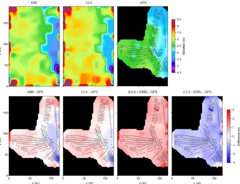
Figure 10.Elevation maps showing the bedrock surfaces detected by the known interface method (KIM) and guided clustering method (CLS) usingbw=0.30. The GPS measured bedrock surface (taken as the ground truth) is also shown. The bottom row shows the corresponding differences between the detected and ground truth bedrock for the two methods, and the limits of uncertainty of the CLS surface, where the error ERR is taken to be half the FWHM of the fuzzy uncertainty distribution around the interface.

the models produced by the two different clustering approaches. Additionally, a model displaying the uncertainty of final chosen fuzzy subset for each clustering is given. The uncertainty was taken to be the complement of the membership value to the final cluster of each data point.

The same process of clustering was applied to the Willington site. In this case, the automated bandwidth selection produced a pdf with three clusters, but again a second bandwidth was manually determined to match the number of clusters to the major formations at the site (terrace deposits overlying clay bedrock). The difference between the bandwidths is smaller in this case, as can be seen in

Fig. 6which shows the pdfs from the two approximations. Peaks

have been identified on the plots and correspond with the centroids used to guide the clustering.Figs 7and8show models with the 2-and 3-clusterings 2-and their respective fuzzy uncertainty.

In bothFigs 4and7, where automated bandwidth is used, more

than one interface is present. These are all shown as clustering surfaces, but none of them are selected to represent the bedrock. Conversely, for the 2-clustering results (Figs 5and8), there is only a single surface separating the clusters, which is assumed to represent the interface between the deposit and the bedrock. In these figures, the single surface is coloured based on its elevation to highlight the

topography. For the more detailed analysis of Willington results, the only continuous clustering interface for the automated bandwidth model is assumed to represent the bedrock and is compared to the interface from the manual bandwidth results inFig. 9.

Smoothing of the automated bandwidth density estimations is necessary due to the nature of the algorithm used. This typically selects a relatively small bandwidth that gives a good global fit to the data but picks out an increased number of potentially insignifi-cant populations. A simple smoothing algorithm (moving average) has given positive results for removing these fluctuations while leav-ing larger significant populations present. A similar issue arises in the choice of bin sizes for the data histograms, where too small a bin range can lead to unwanted detail. In both cases, matching the number of distributions to the expected number of major forma-tions has produced better results for estimating the bedrock surface. However, in cases where less ground truth is available or where the deposit is known or suspected to be highly variable, the automated estimates will provide a useful ‘first look’ analysis of the images.

InFig. 10, a comparison of the detected bedrock for the manual

bandwidth cluster model with the GPS bedrock surface ground truth for Norton Disney is shown. The results are also compared to the

known interface method (KIM; Chamberset al.2013), which uses

by guest on October 19, 2016

http://gji.oxfordjournals.org/

Figure 11. Plots showing detected relative distance (top) and absolute distance from bedrock of KIM (red) and clustering results at multiple known elevations at the Norton Disney site.

Table 1. Willington borehole information with bedrock elevation [m] and comparative values of predicted surface using SGM and guided FCM using kernel bandwidths 0.0318 (automated) and 0.1000 (manually selected). Additionally, for the results from clustering, the full width at half maximum (FWHM) of the uncertainty distribution around the interface is included.

Borehole x y Bedrock SGM bw=0.03 FWHM bw=0.10 FWHM

7 29.50 8.60 21.02 21.22 18.64 0.92 19.15 0.89

8 41.20 8.10 20.76 20.25 16.89 0.80 17.51 0.87

9 49.30 8.44 19.95 20.19 15.39 1.25 16.14 1.20

10 48.50 13.90 19.93 20.23 16.51 0.83 17.01 0.88

11 51.90 8.80 19.83 20.23 15.40 1.22 16.28 1.17

12 54.40 14.00 19.68 20.18 17.13 0.88 17.75 0.89

13 54.50 20.40 20.77 20.21 18.36 0.68 18.73 0.74

14 55.60 33.20 20.73 21.26 19.24 0.51 19.62 0.50

15 27.80 69.20 20.86 21.06 18.59 0.55 18.84 0.54

17 42.20 21.00 19.87 20.27 16.88 0.70 17.25 0.76

18 78.80 7.20 21.76 22.07 20.58 0.55 20.83 0.56

a resistivity isosurface known to intersect the bedrock surface at a chosen point. The distances between the detected surfaces and the GPS surface are shown inFig. 11. The average absolute distances for the clustering and known interface methods are 0.47 and 0.40 m, respectively. An error estimate was derived from the fuzzy uncer-tainty distribution in the vicinity of the interface (Fig. 10). This was taken to be half the full width at half maximum (FWHM) of the uncertainty distribution in the vertical direction. This error estimate had a mean of 0.80 m and a standard deviation of 0.26 m across

the model space. In the bottom rightmost two images inFig. 10,

it can be seen that the error limits effectively bracket the bedrock interface, showing that the bedrock has been detected to within the limits of accuracy of the clustering method.

For the Willington site, it was known that the KIM would not ac-curately detect the interface due to the variability of the deposit (Hsu et al. 2010; Chambers et al. 2012). However, a steepest gradient method (SGM) was found to be applicable in this case

(Chamberset al.2012). The SGM results are compared with the

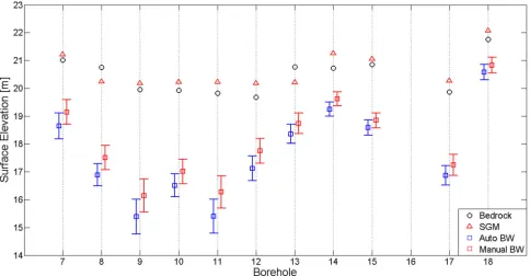
guided clustering method surfaces for both two and three clusters. This comparison does not cover the whole site as ground truth is only known from borehole logs at 11 locations.Table 1andFig. 12 give the results and the FWHM for the clustering surface estimates (these are shown as error bars inFig. 12). For this site, the SGM produced results very close to the interfaces detected in the bore-holes but the clustering results did not agree to within their error estimates. This is because the guided clustering method produces resistivity isosurfaces which, like the KIM, do not work well if the deposit is variable (Chamberset al.2012found that the inverted model resistivity values at the 11 drilling interface locations ranged from 42 to 520m). Due to the heterogeneity of the model, there are some discrepancies, similar to the issues identified in Chambers

et al.(2013) when using the KIM algorithm. It was found that a resistivity isosurface cannot be expected to delineate the mineral in such data, suggesting that the error does not lie in the method.

by guest on October 19, 2016

http://gji.oxfordjournals.org/

320 W.O.C. Wardet al.

Figure 12.Plot showing detected elevations of bedrock (circle) and three methods on the Willington data at borehole sites. The methods shown are steepest gradient method (triangle) and guided clustering using automated bandwidthbw=0.0318 (blue square) and manually selectedbw=0.10 (red square). The error bars are given as half of the FWTM of uncertainty about the interface at each point.

This is highlighted inFig. 12, and shows that even within the fuzzy uncertainty of clustering, the results do not coincide with borehole data.

5 D I S C U S S I O N A N D C O N C L U S I O N

Guided fuzzy clustering has been applied to 3-D ERT images of sand and gravel deposits to detect the interface between the deposit and the bedrock. The method is, however, independent of the spatial dimension of the data and could equally be applied to similar 2.5-D images (e.g. Hsuet al.2010).

The use of fuzzy clustering addresses uncertainty in the mod-els, and reduces the impact of gradational interfaces that can cause problems with gradient-based interface detection on certain sites

(Chambers et al. 2013). When compared to other methods that

attempt to assign resistivity isosurfaces to formation interfaces

(Chambers et al. 2013), considerably fewer assumptions were

needed in the guided fuzzy clustering approach. Knowledge of the expected number of major formations was sufficient to achieve good results; otherwise, there was little user intervention. Even when manually selecting bandwidths, a plot of the pdf provides an easily accessible visualization of the feature space regardless of the size and dimension of the input data.

In terms of runtime efficiency, the original FCM algorithm runs

at O(cbN), where N is the number of data,cis the number of

clusters and b is the number of iterations required to converge:

bincreases in magnitude with the increase of dimension. The iter-ation limit,bmax, is typically chosen to be 1000 for a 3-D data set,

although convergence does not often occur. With the distribution-guided clustering introduced in this paper, the framework runs at

O(cN), with KDE and local maxima detection running at O(N). For the given examples, the algorithm takes approximately 1 min to run on a dual Intel Xeon E5620 system.

Limitations of this approach fall largely into two categories: lim-itations of resistivity imaging and limlim-itations of the edge detection methods. The former include the exponential decrease of resolu-tion with distance from the electrodes and the gradaresolu-tional nature of interfaces produced by smoothness-constrained inversion. The edge detection algorithm involved KDE and FCM to identify the inter-faces, which discard any spatial information. It may be possible to improve the results by incorporating summation of the mem-bership function over a defined neighbourhood of each cell under

consideration (Chuanget al.2006). While the means taken from

KDE were identified as population centroids, no other distribution information was used. Using the trough locations of the pdf to approximate, the standard deviation of each population could give a means of further guiding the clustering approach by incorporating it into the FCM weighting function.

An extension of the methods presented in this paper could follow multiple directions. One of the more simple possibilities includes applying the methods to higher dimensional data, such as 4-D (time-lapse) ERT monitoring of sites. A further improvement of the methods could be made by incorporating data from other geophysical survey methods (Ellefsenet al.1998). This could be achieved by adapting multivariate versions of both fuzzyc-means

and KDE (Gustafson & Kessel1978; Silverman1986; Simonoff

1996). This may further isolate deposits and would perhaps increase the capability of classification.

A C K N O W L E D G E M E N T S

We thank the editor and two anonymous reviewers for their helpful comments on our original manuscript. The data used in this paper were acquired by a project funded by Defra through the MIST Programme (grant MA/7/G/1/007) and in-kind contributions from

by guest on October 19, 2016

http://gji.oxfordjournals.org/

Barron, A.J.M., Sumbler, M.G., Morigi, A.N., Reeves, H.J., Benham, A.J., Entwisle, D.C. & Gale, I.N., 2010. Geology of the Bedford district— a brief explanation of the geological map, 1:50 000 Sheet 203 Bedford (England and Wales).

Berridge, N.G., Pattinson, J., Samuel, M.D.A., Brandon, A., Howard, A.S., Pharoah, T.C. & Riley, N.J. 1999. Geology of Grantham district. Memoir of the British Geological Survey, Sheet 127 (England and Wales). B¨ohm, G., Brauchler, R., Nieto, D.Y., Baradello, L., Affatato, A. & Sauter,

M., 2013. A field assessment of site-specific correlations between hy-draulic and geophysical parameters,Near Surf. Geophys.,11,473–483. Boreham, S., White, T.S., Bridgland, D.R., Howard, A.J. & White, M.J.,

2010. The Quaternary history of the Wash fluvial network, UK,Proc. Geol. Assoc.,121,393–409.

Botev, Z., Grotowski, J. & Kroese, D., 2010. Kernel density estimation via diffusion,Ann. Stat.,38,2916–2957.

Bridgland, D.R., 2006. The middle and upper Pleistocene sequence in the lower Thames: a record of Milankovitch climatic fluctuation and early human occupation of southern Britain—Henry Stopes Memorial Lecture 2004,Proc. Geol. Assoc.,117,281–305.

Cannon, R.L., Dave, J.V. & Bezdek, J., 1986. Efficient implementation of the fuzzy c-means clustering algorithms,IEEE Trans. Pattern Anal. Machine Intell.,2,248–255.

Chambers, J.E.et al., 2012. Bedrock detection beneath river terrace deposits using three-dimensional electrical resistivity tomography, Geomorphol-ogy,177,17–25.

Chambers, J.E., Wilkinson, P.B., Penn, S., Meldrum, P.I., Kuras, O., Loke, M.H. & Gunn, D.A., 2013. River terrace sand and gravel deposit reserve estimation using three-dimensional electrical resistivity tomography,

J. appl. Geophys.,93,25–32.

Chuang, K.-S., Tzeng, H.-L., Chen, S., Wu, J. & Chen, T.-J., 2006. Fuzzy c-means clustering with spatial information for image segmentation,

Comput. Med. Imag. Graphics,30,9–15.

Dahlin, T. & Zhou, B., 2004. A numerical comparison of 2D resistivity imaging with 10 electrode arrays,Geophys. Prospect.,52,379–398. Ellefsen, K.J., Lucius, J.E. & Fitterman, D.V., 1998. An evaluation of several

geophysical methods for characterising sand and gravel deposits, Open-File Report 98-221, U.S. Geological Survey.

Estivill-Castro, V., 2002. Why so many clustering algorithms: a position paper,ACM SIGKDD Explor. Newslett.,4,65–75.

Gharibi, M. & Bentley, L.R., 2005. Resolution of 3-D electrical resistiv-ity images from inversions of 2-D orthogonal lines,J. Environ. Eng. Geophys.,10,339–349.

Green, C.P.et al., 1996. Pleistocene deposits at Stoke Goldington, in the valley of the Great Ouse, UK,J. Quatern. Sci.,11,59–87.

3-D fluvial architecture and grain-size distribution of a gravel flood-plain in northeast British Columbia, Canada,J. Sediment. Res.,79,457– 477.

Hirsch, M., Bentley, L.R. & Dietrich, P., 2008. A comparison of electrical resistivity, ground penetrating radar and seismic refraction results at a river terrace site,J. Environ. Eng. Geophys.,13,325–333.

Horton, A., 1970. The drift sequence and sub-glacial topography in parts of the Ouse and Nene Basins,Report of the Institute of Geological Sciences 70/9,HMSO, London.

Hsu, H.L., Yanites, B.J., Chen, C.C. & Chen, Y.G., 2010. Bedrock detection using 2D electrical resistivity imaging along the Peikang River, central Taiwan,Geomorphology,114,406–414.

Lanh, T.T., 1990. Kernel density estimation under dependence,Stat. Probab. Lett.,10,193–201.

Loke, M.H., Acworth, R.I. & Dahlin, T., 2003. A comparison of smooth and blocky inversion methods in 2D electrical imaging surveys,Explor. Geophys.,34,182–187.

Loke, M.H. & Barker, R.D., 1996. Practical techniques for 3D resistivity surveys and data inversion,Geophys. Prospect.,44,499–523.

Loke, M.H., Chambers, J.E., Rucker, D.F., Kuras, O. & Wilkinson, P.B., 2013. Recent developments in the direct-current geoelectrical imaging method,J. appl. Geophys.,95,135–156.

MacQueen, J., 1967. Some methods for classification and analysis of multi-variate observations, inProceedings of the Fifth Berkeley Symposium on Mathematical Statistics and Probability,vol.1,pp. 281–297.

Rogerson, R.J., Keen, D.H., Coope, G.R., Robinson, E., Dickson, J.H. & Dickson, C.A., 1992. The fauna, flora and palaeoenvironmental signifficance of deposits beneath the low terrace of the River Great Ouse at Radwell, Bedfordshire, England, Proc. Geol. Assoc., 103,

1–13.

Rosenblatt, M., 1956. Remarks on some nonparametric estimates of a density function,Ann. Math. Stat.,27,832–837.

Sass, O., 2007. Bedrock detection and talus thickness assessment in the European Alps using geophysical methods,J. appl. Geophys.,62,254– 269.

Sheather, S.J. & Jones, M.C., 1991. A reliable data-based bandwidth selec-tion method for kernel density estimaselec-tion,J. R. Stat. Soc. B,53,683–690. Silverman, B.W., 1986.Density Estimation for Statistics and Data Analysis,

Vol. 26, Chapman & Hall/CRC.

Simonoff, J.S., 1996.Smoothing Methods in Statistics,Springer.

Wilkinson, P.B., Loke, M.H., Meldrum, P.I., Chambers, J.E., Kuras, O., Gunn, D.A. & Ogilvy, R.D., 2012. Practical aspects of applied optimised survey design for electrical resistivity tomography,Geophys. J. Int.,189,

428–440.

by guest on October 19, 2016

http://gji.oxfordjournals.org/