July 2012, Volume 3, Issue 7. http://www.jenvstat.org
Using INLA To Fit A Complex Point Process Model
With Temporally Varying Effects – A Case Study
Janine B. Illian
University of St Andrews
Sigrunn H. Sørbye
University of Tromsø
H˚avard Rue
Norwegian University of
Science and Technology,
Trondheim
Ditte Hendrichsen
Aarhus University, and
Norwegian Institute for
Nature Research,
Trondheim
Abstract
Integrated nested Laplace approximation (INLA) provides a fast and yet quite exact
approach to fitting complex latent Gaussian models which comprise many statistical models
in a Bayesian context, including log Gaussian Cox processes. This paper discusses how a
joint log Gaussian Cox process model may be fitted to independent replicated point patterns.
We illustrate the approach by fitting a model to data on the locations of muskoxen (Ovibos
moschatus) herds in Zackenberg valley, Northeast Greenland and by detailing how this
model is specified within the R-interface R-INLA. The paper strongly focuses on practical
problems involved in the modelling process, including issues of spatial scale, edge effects and
prior choices, and finishes with a discussion on models with varying boundary conditions.
1. Introduction
Integrated nested Laplace approximation (INLA) provides a fast and yet quite exact approach
to fitting latent Gaussian models which comprise many statistical models, including models
with temporal or spatial dependence structures (Rue, Martino, and Chopin 2009). As a result,
many complex models that previously required the use of time-consuming Markov chain Monte
Carlo (MCMC) calculations can be fitted fast and conveniently. Log Gaussian Cox processes,
a particularly flexible class of spatial point process models are a special case of latent Gaussian
models. Rue et al. (2009),Illian, Sørbye, and Rue (2012) and Illian and Rue(2010) show that
complex point process models, including hierarchically marked point processes may conveniently
be fitted with INLA. Standard approaches to parameter estimation for complex models based
on MCMC, for example, would be very cumbersome and computationally prohibitive.
Fitting spatial point process models to some spatial patterns is computationally intensive due
to – amongst other things – the large number of individual points in the data set (Burslem,
Garwood, and Thomas 2001;Waagepetersen 2007;Waagepetersen and Guan 2011;Law, Illian,
Burslem, Gratzer, Gunatilleke, and Gunatilleke 2009). Here, we consider a rather different
situation. In some applications difficulties arise since point patterns with only a very small
number of points can be collected, due to logistic limitations (e.g. for reasons of accessibility).
These patterns are sometimes too small to justify the modelling of a single pattern. However, if
replicates exist, a joint model of all replicates with a factor that accounts for variability among
replicates caused by different conditions on different days may be more suitable. Mixed effect
models for replicated point patterns have recently been considered in a frequentist approach
for Gibbs processes (Illian and Hendrichsen 2010). In that approach, parameter estimation
was based on the pseudolikelihood of a Gibbs process as well as maximum quasi-likelihood
optimisation. Here we discuss how data with a similar structure may be modelled with a log
The data that we have available have been collected at different time points and hence we
consider a complex point process model with a temporally varying effect and construct a model
that may then be fitted with INLA. This approach provides us with more general modelling
facilities that allow us to fit several models of varying complexity and compare their suitability
for a given data set. We show in detail how this model is specified in practice, within the
R-interface R-INLA (available at www.r-inla.org), and discuss issues involved in fitting the
model to a data set derived from an ecological field study. We use a data set detailing the
locations of muskoxen herds in Greenland (Illian and Hendrichsen 2010; Schmidt, Berg, and
Meltofte 2010) to illustrate the approach. In addition, we discuss issues of fitting log Gaussian
Cox processes to point patterns that have been observed in observation windows where some
of the edges are real edges (Illian, Penttinen, Stoyan, and Stoyan 2008) which is particularly
common in animal studies.
2. Modelling approach
2.1. The data
We consider a situation whereT point patternsx1, . . . ,xT have been observed in an observation
windowSat different points in time,t= 1, . . . , T. The objects represented by the points may be
considered independent of the objects observed at other points in time conditional on common
observed (spatial) covariatesz1, . . . , zpand other unobserved covariates. The pattern may differ
between the different time points as a result of observed and unobserved influences specific to
a given point in time. In order to fit a single model to all replicates, “time” may be treated as a
factor in a point process model. For illustration, the approach is applied to a data set detailing
the spatial locations of muskoxen (Ovibos moschatus) herds in Zackenberg valley, Northeast Greenland, 74◦300N – 21◦000W (hereafter referred to as “muskoxen data”) at different points in
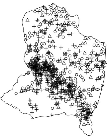
the study area within Greenland and Figure1 C for a map of the area.
[Figure 1 about here.]
The muskoxen at Zackenberg have been studied since 1996 as part of a large-scale monitoring
programme in the area (Meltofte, Christensen, Elberling, Forchhammer, and Rasch 2008). The
census area covers 45 square km, ranging from sea level to 600 masl. The spatial locations
of muskoxen herds have been recorded weekly during the summer months, July and August,
occasionally also in June. During the censuses, all herds within the census area have been
mapped to the nearest 100 metres (Schmidt et al. 2010), then approached and identified to
age and sex followingOlesen and Thing (1989). The categories are calves, yearlings, two-year,
three-year and four-years or older. There is an interest in analysing the spatial distribution of
muskoxen in relation to spatial covariates such as altitude or an index of vegetation productivity,
the normalized differential vegetation index (NDVI).
In this paper we analyse a subset of the muskoxen data corresponding to the years 2005–2007.
The observed locations of the muskoxen herds across all time points during these years are
illustrated in Figure 2, indicating that the intensity of the patterns seems to be particularly high
in one specific area that forms a diagonal across the plot. Illian and Hendrichsen(2010) model a
similar data set with a Gibbs process and fit the model by approximating the pseudolikelihood
based on a generalised linear mixed model with Poisson outcome. They include “time” as a
random effect applying the approximate Berman-Turner device (Baddeley and Turner 2000)
in a frequentist approach. Here we specify a log Gaussian Cox process model and fit it in a
Bayesian context, an approach that allows more flexibility and makes the fitting and comparison
of several models of varying complexity feasible.
2.2. Model fitting in INLA
A log Gaussian Cox process is a hierarchical Poisson process with random intensity Λt(s) =
exp{ηt(s)}, where ηt = {ηt(s) : s ∈ Rd} denotes a Gaussian field. This type of model is
a special case of the more general class of latent Gaussian models, for which deterministic
Bayesian inference can be performed using the INLA-methodology, seeRue et al. (2009).
In general, latent Gaussian models can be described as a subclass of structured additive
regres-sion models, in which the predictor can be expressed in terms of linear and non-linear effects of
covariates. Explicitly, the meanµj =E(yj) of observations is linked to a predictor
ηj =g(µj) =β0+
X
α
βαzjα+
X
γ
fγ(cjγ), (1)
whereβ0denotes an intercept, while the sets{βα}and{fγ(.)}denote linear effects of covariates
{zα}and non-linear effects of covariates {cγ}, respectively. By assigning Gaussian priors to all
random terms in (1), we obtain a latent Gaussian model.
Here, we fit a log Gaussian Cox process to a specific two-dimensional point patternxtdiscretising
the observation windowS intoN grid cells{si}Ni=1, where each cell has area|si|. For each time
point t = 1, . . . , T, let yti denote the observed number of points in grid cell si. Conditional
on the intensities Λt(si) = exp{ηt(si)}, the joint pattern of replicates can be described as a
superpositionx=S
t=1,...,Txt of realisations from independent Poisson processes, where
yti|ηt(si)∼Po(|si|exp(ηt(si))).
We assume that the log-intensity of the Poisson processes can be described by the linear predictor
ηt(si) =β0+βt+
X
α
βαztα(si) +
X
γ
fγ(ctγ(si)), (2)
in which the off-set β0 represents an intercept common to all time points while the factor βt
accounts for variation in intensity across different time points. As in (1), the set{βα} accounts
We also include potentially smooth effects of covariates{ctγ(.)}, in which the functions{fγ(.)}
are estimated based on all replicates.
The primary aim in using the INLA-methodology is to find posterior estimates of all the random
terms in the log-intensity in (2), numerically. These terms are collected in a latent field ζ =
{β0, βt,{βα},{fγ(.)}}, and assigned Gaussian priors such that the resulting model can be viewed
as a latent Gaussian model. The posterior marginals of each element ζj of the latent field can
be expressed by
π(ζj |y) =
Z
π(ζj |θ,y)π(θ|y)dθ, (3)
where the vectorθdenotes the hyperparameters of the model. Here, θincludes the parameters
used in defining prior distributions for the precision (inverse variance) of the Gaussian priors,
in which
π(θj |y) =
Z
π(θ|y)dθ−j. (4)
Applying the INLA-methodology, the marginals in (3) - (4) are estimated combining analytical
approximations with numerical integration, see Rue et al. (2009) for a thorough description.
The first step in this procedure is to estimate π(θ | y) using a Laplace approximation. The
Laplace approximation is defined by
˜
π(θ|y)∝ π(ζ, θ,y)
˜
πG(ζ |θ,y)
ζ=ζ∗(θ)
,
where the full conditional of the latent field is approximated by a Gaussian distribution ˜πG(ζ |
θ,y), evaluated at the mode ζ∗(θ). Secondly, estimates of the marginals π(ζj | θ,y) in (3)
can be found either using a Laplace or a simplified Laplace approximation. Alternatively, the
marginals can be estimated using a Gaussian approximation derived from ˜πG(ζ |θ,y). Although
the Gaussian approximation might provide some inaccuracies in estimating the marginals (Rue
and Martino 2007), this approach is used here to speed up calculations.
The third and final step in approximating the marginals of the latent field is to use numerical
numerically to find support points for the numerical integration. The resulting approximation
to (3) is given by
˜
π(ζj |y) =
X
k
˜
πG(ζj |θk,y)˜π(θk|y)∆k,
where ˜π(θk | y) is found by numerical integration in (4) and ∆k denotes the area weight
corresponding to integration point θk. The resulting approximation has been shown to be very
accurate (Rueet al. 2009) and is also computationally much more efficient than using
MCMC-approaches.
2.3. Specifications for the muskoxen data set
In fitting (2) to the given subset of the muskoxen data, we have considered two observed
en-vironmental covariates, the altitude and the normalized differential vegetation index (NDVI).
The vegetation index is not available for all time points, including the years 2006 and 2007. In
various submodels for individual years this covariate has turned out to be non-significant and
is hence not included in the final model.
To account for small scale spatial variation not caused by environmental covariates but by
inter-individual (or here: inter-herd) interactions, we apply the ideas in Illianet al. (2012) and
introduce a constructed covariate in (2), that relates each midpoint of cell si ∈ S to pattern
points in the neighbourhood. Specifically, for grid cell si we define the constructed covariate
ct(si) to be the Euclidean distance from the midpoint mi of cell si to the nearest point xtj in
the pattern outside si at time point t, i.e.
ct(si) = min
xtj∈xt\si
(|mi−xtj|)
where|.|denotes the Euclidean distance. However, for each time point the constructed covariate
for cell si is defined to be missing if the distance ct(si) is larger than the minimum Euclidean
distance between mi and the border, see section 2.5 for remarks on potential edge effects.
Section2.4for further discussions on the choice of the constructed covariate. It is incorporated
in (2) using a smooth function fcc(.) as the functional relationship between the intensity and
the constructed covariate may not be linear. Specifically, the function fcc(.) is modelled using
a first-order conditional autoregressive (CAR) model, applying a gamma prior for the precision
parameter. Similarly, large-scale spatial variation is included in (2) as a smooth function in
space fspat(.) for all the grid cells and across all time points. Here, the spatial function is
specified as a second-order two-dimensional CAR-model on a lattice, as this spatial model is
supported by R-INLA. A gamma prior is used also for the precision parameter of the spatial
model, see Section2.4and 3.1for a discussion on appropriate choices for the prior parameters.
The resulting model for the muskoxen data set can be summarised as
ηt(si) =β0+βyear+β1z1(si) +fday(t) +fcc(ct(si)) +fspat(si), t= 1, . . . , T, i= 1, . . . , N, (5)
where z1(.) denotes the altitude for the different grid cells. We have modelled the temporally
varying effect by a factorβyear accounting for the yearly increase in mean intensity observed for
the years 2005 - 2007. In addition, we include a smooth functionfday(t) assuming independent
Gaussian observations, which accounts for random variation in intensity on different days. To
ensure identifiability of the intercept, all of the smooth functions are constrained to sum to zero.
2.4. Issues of spatial scale – prior choices
In an analysis of a spatial pattern, it is crucial to bear in mind the spatial scales that are relevant
for a specific spatial data set. Here we assume that social behaviour among the herds operates
at a local spatial scale and that the association with environmental covariates operates on the
scale of the variation in these covariates and hence often on a larger spatial scale.
The large-scale spatial effect in (5) is included as a spatially structured error term to account for
any spatial autocorrelation unexplained by covariates in the model. The choice of the gamma
effect and, through this, the spatial scale at which it operates. To avoid overfitting, and in
order to obtain a model describing a generally interpretable trend we choose the prior so that
the spatial effect operates at a similar spatial scale as the covariate. This ensures that the
spatially stuctured effect does not operate on a smaller scale than the covariate as it would
otherwise be likely to explain the data better than the covariates, rendering the model rather
pointless. We approach this by repeatedly fitting a simple model (see Section 3.1), comparing
the estimated spatial effect to a plot of the covariate.
If small scale inter-individual spatial behaviour is of specific interest in an application it may
be modelled by the constructed covariate to account for local spatial behaviour. The muskoxen
herds are likely to interact mainly with the herd that is closest to them (Dice 1952;Clark and
Evans 1955) and so the distance to the nearest neighbour has been chosen here as a constructed
covariate accounting for local behaviour. This is of interest since the model may be used to
reveal the relevant distances at which the herds interact. Again there is a danger of overfitting,
especially since the constructed covariate is estimated directly from the point pattern. Illian
et al. (2012) discuss practicalities of using a spatial constructed covariate and point out the
importance of the choice of the covariate and its relevance to the specific application. Note
that Cox processes are unable to model dependence between points. We have attempted to
cir-cumvent this limitation by using a constructed covariate implicitly assuming that local spatial
structures captured by the covariate are the result of an underlying process that has not been
observed directly. In other words, we do not assume that the observed patterns were generated
by a mechanism that includes the constructed covariate (in which case it would no longer be
a Cox process) but that the constructed covariate is a proxy for an unknown latent variable
that reflects local structure. This assumption is clearly justified in the example discussed in
Illianet al.(2012), where the constructed covariate mimics local seed dispersal (and hence some
function of the distance from the parent tree). In the muskoxen data set, the Cox process
inde-pendent. It is certainly less obvious why this assumption may be made here as one might prefer
to interpret local structures as resulting from direct interactions among the herds rather than
from a location dependent random field. However, the approach we take here is currently the
only way to incorporate local structures into a complex model that may be fitted with INLA.
The choice of grid size is also linked to issues of spatial scale. Here we apply the same grid and
grid resolution as used in the data collection of locations of the muskoxen herds.
2.5. Edge effects and boundary conditions
Spatial point pattern data are usually observed in a finite observation window only. Since there
typically is no data about the behaviour of the pattern outside the window, edge effects occur
and often have to be accounted for (Illianet al.2008), in particular in the context of stationary
point processes. Edge effects have only a minor impact on large point pattern data sets such as
the rainforest data discussed in Rue et al.(2009).
However, in smaller data sets, including the data considered here, edge effects are certainly
relevant. Here, we consider a data set observed within a polygonal window assuming that Λt(.)
is defined in R2, i.e. that if the pattern had been observed beyond any of the edges it would
have the same properties as inside the observation area. For simplicity, we currently assume
that all edges are of the same quality, i.e. that they have been arbitrarily chosen and have no
impact on the spatial pattern. In applications this is not necessarily the case as the boundary
may reflect a true barrier beyond which the conditions are very different. This might imply that
the pattern does not continue in exactly the same way and that, more importantly, the barrier
has a direct influence on the pattern near the edge. We consider these issues in the discussion
in Section 4.3 indicating potential approaches to solving these.
It is necessary to account for potential edge effects in the constructed covariate leading to an
overestimation for cells close to the boundary as there might be points outside the observation
calculation of the constructed covariate we hence exclude all cells for which the distance of
its midpoint to the nearest point in the pattern is larger than its minimum distance to the
boundary.
3. Results
To illustrate the modelling approach we consider a subset of the muskoxen dataset, consisting
of the patterns collected on T = 26 different days. The observation period included weekly
observations for a total of 10, 7 and 9 days during the summers of 2005 - 2007, respectively.
Across the years, the subset consists of a total of 754 observed muskoxen herds. These are likely
to include repeated observations of the same muskoxen herds at different time points. Since
information on herd identity is not available we cannot account for this in the model.
In discretizing the given observation window S, we apply the same grid as used in collecting
the data, in which herds within the area were mapped to the nearest 100 metres (Schmidt
et al. 2010). This gives a total of N = 4533 grid cells, each having an area equal to 0.01
km2. Technically, the joint model for all locations and replicates is run in R-INLA stacking all
observations in one vector y ={yti, t = 1, . . . , T, i = 1, . . . , N}, having corresponding vectors
for the other terms in the model. Consequently, for the given subset of the data, the length of
these vectors is 117858. We fit the model in (5) to the data and apply the deviance information
criterion (DIC) (Spiegelhalter, Best, Carlin, and der Linde 2002) to assess the importance of
the different terms in the model.
3.1. Prior choices
We initially fit a very simple model to the data where we explain the location of the herds purely
based on a common spatial effect for all time points. This is done to assess the resolution of the
spatial effect and simplify prior choice. We fit the model repeatedly using different values for
We deliberately choose the prior for the spatial effect manually as assessing the model based on
DIC would encourage overfitting. Clearly, prior choices for the parameters could be done using
the full model in equation (5) as well, but this would be more time-consuming.
We apply the simple model
ηt(si) =β0+fspat(si), (6)
which takes about 15 seconds to run for each of the different parameter choices. The call in
R-INLA to fit this simple model is
> formula = y ~ 1 + f(i.spat, model = "rw2d", nrow = nrow, ncol = ncol,
hyper = list(prec = list(param=prior.spat)))
> result = inla(formula, data=data, family = "poisson",
control.inla = list(strategy = "gaussian"), control.compute=list(dic=TRUE))
The1in the call specifies a common intercept, whilef(i.spat)represents the smooth function
of the spatial effect fspat(si). The spatial model is specified as a second-order CAR-model on
a lattice. In R-INLA this model is referred to as (rw2d), here having dimension nrow×ncol
which covers the observation window. The shape and scale parameter of the gamma distribution
used as a prior for the hyperparameter, being the precision of the spatial model, is given as the
parameter vector prior.spat. Clearly, the function call to INLA bears strong resemblance to
that familiar from other functions in well-known R libraries, such as lm or glm, and as in the
latter, the model family has to be given as family = "poisson". Due to the size of the final
model we apply the Gaussian approximation to estimate the marginals of each component of
the latent field (strategy=gaussian). Also, we specify that the DIC value should be calculated
(dic=TRUE).
Figure 3 illustrates how the spatial effect varies with different prior choices for the
hyperpa-rameter. We compare the smoothness of the estimated surface to that of the observed altitude
The spatial effect reflects very local behaviour (clustering at a smaller scale than the empirical
covariate) and hence potentially yields a model that is overfitted to the given observations, see
Figure3(b). In Figure3(c), a moderate degree of smoothing is obtained using the parameters
(40, 0.001), in which the spatial effect clearly indicates the higher intensity of points in the
central area that is also obvious from the plot of the pattern. A similar degree of smoothness
results for a quite wide range of prior parameters and hence this prior has been chosen for the
analysis of the full model. Figure3 (d) shows the estimated spatial effect using the parameters
(100, 0.001), leading to a very smooth spatial effect which seems too strong for the current
application.
[Figure 3 about here.]
We take a similar approach to determine the prior for the constructed covariate and again fit a
simple model to the data and observe how the smoothness of the estimated function varies with
the choice of prior parameters. The model we fit here contains only the constructed covariate
and a common intercept, such that
ηt(si) =β0+fcc(ct(si)). (7)
Figure 4 (a) indicates that using a gamma prior with parameters (2, 0.01), results in a very
wiggly curve. This is likely to be due to uninformative noise and stronger smoothing of the
curve is required. The choice of prior parameters (60, 0.01), yields a much smoother curve, see
Figure4(b). The estimated curve looks very similar for quite a wide range of prior parameters
and this set of priors has been chosen for the final analysis. Finally, the effect of choosing an
extreme prior becomes clear in Figure4(c) with parameters (2000, 0.01) which results in a very
smooth and much flatter curve.
3.2. Model selection
Informed by the fit of the simple model in equation (6) we choose the prior parameters for the
spatial effect asprior.spat = (40,0.001) and fit the full model in (5) to the muskoxen dataset.
The formula specification to run this model in R-INLA has the following format,
> formula = y ~ year.factor + cov.alt + f(day, model = "iid") +
f(inla.group(cov.cc), model = "rw1", hyper = list(prec = list(param = prior.cc))) +
f(i.spat, model = "rw2d", nrow = nrow, ncol = ncol,
hyper = list(prec = list(param = prior.spat)))
The model took 213 seconds to run on a 12 core 2.33 GHz machine and the DIC for this
model is 8515. By specifying the year factor with three levels, we estimate a common
inter-cept ˆβ0 = −5.108. The additionally estimated coefficients for the years 2006 and 2007 are
ˆ
βyear = (0.108,0.505), accounting for the increase in observed muskoxen herds during these
years. Having accounted for the annual effect, the estimated temporal effect as a function of
days was seen to be negligible. The altitude (specified by cov.alt), has a significant negative
effect on the intensity of the points with an estimated mean equal to−0.006 with a 95% credible
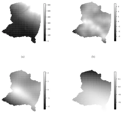
interval given by (−0.007, −0.004), see Figure 5 (a) for the resulting estimated effect of
alti-tude. The plot of the constructed covariate clearly indicates local clustering (Figure5(b)). The
estimated spatial effect (Figure 5 (c)) shows a smooth and non-constant surface. This surface
might suggest other factors that have not been considered in the model (or in the overall study)
but may influence the pattern. Most markedly, in the south west corner fewer herds appear to
have been observed than the covariate altitude can explain.
[Figure 5 about here.]
In order to assess the effect of the various terms in (5), we repeatedly fit submodels of the full
[Table 1 about here.]
In concrete applications several covariates are often available and the DIC may be used to
identify the best model in terms of the covariates considered. We notice that DIC for a model
without the year and day effects is clearly higher than the full model supporting the inclusion
of the time-varying effect in the model. Likewise, the model without the altitude covariate
leads to a DIC of 8558, clearly indicating that the model may be improved by including this
covariate. Table 1 also illustrates that both the inclusion of a constructed covariate and a
large-scale spatial effect improves the model as the spatial autocorrelation cannot be explained fully
by the covariate.
4. Discussion
In many areas of science, rapidly improving technology facilitates data collection these days.
Ecologists in particular, have become aware of the importance and relevance of spatial
infor-mation for an understanding of population dynamics. For these reasons, spatially explicit data
sets have become increasingly available in ecology as well as many other areas of science,
in-cluding geosciences, molecular genetics, evolution and game theory with the aim of answering a
similarly broad range of scientific questions. Currently, these data sets are often analysed with
methods that either do not account for spatial autocorrelation or that do not make full use
of the available spatially explicit information, which might provide interesting information on
spatial processes. In the context of spatial point pattern data, methodology needs to be made
available as well as accessible to applied scientists by facilitating the fitting of suitable models to
help provide answers to concrete scientific questions. In order to address this issue, this paper
illustrates in detail the process of fitting a specific spatial point process model to a realistically
complex data set using modern model fitting methodology. This provides non-specialists with
models accessible.
In the specific case considered here, a simple analysis of each of the patterns that does take
the spatially explicit information into account would not be sufficient. The small size of the
individual patterns would render this analysis rather uninformative such that a complex joint
model of several subpatterns has to be considered in order to gain an understanding of the
system. In particular, to be able to fit this complex model we apply the deterministic Bayesian
INLA-methodology, to fit a model to a replicated point pattern allowing for variation among
the replicates by considering time-varying effects. The INLA approach speeds up parameter
estimation substantially such that we can fit several models within feasible time and use model
comparison methods to identify the most suitable model.
4.1. Model comparison and assessment
The modelling approach provides methods of model comparison through the DIC so that it
was possible to identify the most suitable model for the specific data set and to avoid
over-parameterisation.
The fact that NDVI does not adequately explain the spatial distribution of muskoxen here is
likely due to insufficient information in the covariate as measured for the current study. The data
were collected on a single day at the start of the season and are hence may not sufficiently reflect
the environmental conditions later in the season. In general, NDVI has become increasingly
popular as a measure of primary production. It is highly correlated with herbivore distribution
at larger scales (Pettorelli, Gaillard, Mysterud, Duncan, Stenseth, Delorme, Laree, To¨ıgo, and
Klein 2006), and has become a useful tool in explaining herbivore distribution and movement
in areas where direct measurements of vegetation variables such as biomass and quality is not
available. We are are in the process of acquiring data that provide information on greenness on
a given day. This information that accounts for changes in vegetation throughout the season
in the habitat preferences of the muskoxen herds.
Altitude, by contrast, has a strong influence on vegetation communities, and may more
ac-curately capture the variations in vegetation distribution, phenology and green-up (Mysterud,
Langvatn, Yoccoz, and Stenseth 2001), factors which are likely to be of more importance to
muskoxen than the more crude measure of primary productivity.
4.2. Boundary conditions
The current model assumes that all edges of the observation window were artificial edges
deter-mined by the choice of the observation window and hence that the pattern was a sample from
a stationary process that continues in the same way beyond the boundaries. This assumption
is sensible in many data examples, where the observation window is a plot within a larger area
with similar characteristics. For instance, the examples discussed inRueet al.(2009) andIllian
and Rue (2010) consider point patterns in rectangular observation window whose edges have
been arbitrarily chosen. However, strictly speaking, this assumption does not hold for the
con-crete example data set. For example, the southern boundary is formed by the sea and muskoxen
herds would never be observed beyond this border. In some data sets a border like this might
constitute a reflective boundary causing a higher intensity of animals close to it. In other cases,
the animals might actively avoid the vicinity of this boundary.
Muskoxen are highly motile and in principle capable of utilising the entire census area, including
the area immediately bordering the shoreline. However, their incitement to approach the
bound-ary may depend on a number of factors, of which the distribution and quality of the vegetation
is most obvious. The distribution of plant communities is strongly affected by factors such as
soil quality, water and nutrient availability and exposure, all of which may be influenced by
distance to the sea. It is therefore relevant to consider covariates when interpreting the effect of
the boundary. In addition to the absolute nature of the shoreline as a boundary, other sections
an absolute obstacle. For example, large sections of the left hand (western) and right hand
(eastern) boundaries are demarcated by rivers which are passable to muskoxen, but where the
degree of connectivity may vary with season (influencing water discharge and break-up of ice)
and with the age or condition of the animals attempting to cross.
Situations where spatial point patterns have been observed within an observation window with
a true edge have been discussed in the context of finite point processes (Illian et al. 2008).
However, the given data set cannot be treated as a finite point process since it is not a truly
finite process. The animals can move in and out of the area at some parts of the boundary
and, more importantly, these boundaries have been arbitrarily chosen. Hence it is useful to
assume that the pattern continues in the same way beyond some part of the boundary and that
the edge has no effect on the pattern. In other words, a more realistic model of the data than
the model that we currently consider would consider the varying nature of the boundary. This
issue is likely to be relevant in many studies where spatial data on a large spatial scale have
been observed. For practical reasons (e.g. accessibility or ease of data collection) observation
areas are often chosen to line up with existing natural borders which might directly impact
on the spatial behaviour within the resulting observation window. In some applications, the
influence of the edge on the pattern might even be of primary interest to a study. Approaches
that allow the fitting of complex models to data sets with complicated boundary structures are
highly relevant not only to the specific data set discussed here but also to many other data sets
detailing the locations of animals, such as marine mammals (Sveegaard, Teilmann, Tougaard,
Dietz, Mouritsen, Desportes, and Siebert 2011).
Currently, it is not possible to account for different types of edges in INLA. However, the
approaches introduced inLindgren, Rue, and Lindstr¨om(2011) and Simpson, Illian, Lindgren,
Sørbye, and Rue (2011) can be used to incorporate these in a model in a straight forward way
based on stochastic partial differential equations where different boundary conditions may be
be applied to data sets with varying types of boundaries.
5. Acknowledgements
We would like to thank Mads C. Forchhammer, Niels Martin Schmidt and Mikkel Tamstorf from
Greenland Ecosystem Monitoring, National Environmental Research Institute, Aarhus
Univer-sity for making the data available to us. We would also like to thank Finn Lindgren, UniverUniver-sity
of Trondheim and Daniel Simpson, University of Helsinki for many fruitful discussions. Some of
the computations for this paper were run on the RINH/BioSS Beowulf cluster at the University
of Aberdeen, Rowett Institute of Nutrition and Health (http://bioinformatics.rri.518 sari.ac.uk).
We thank Tony Travis for his generosity and assistance.
References
Baddeley A, Turner R (2000). “Practical maximum pseudolikelihood for spatial point processes.”
New Zealand Journal of Statistics,42, 283–322.
Burslem DFRP, Garwood NC, Thomas SC (2001). “Tropical forest diversity – the plot thickens.”
Science,291, 606–607.
Clark PJ, Evans FC (1955). “Distance to nearest neighbor as a measure of spatial relationship
in populations.” Ecology,35, 445–453.
Dice LR (1952). “Measure of the spacing between individuals within a population.” Contrib. Lab. Vert. Biol. Univ. Mich.,55, 1–23.
Illian JB, Hendrichsen DK (2010). “Gibbs point process models with mixed effects.” Environ-mentrics,21, 341–353.
Illian JB, Rue H (2010). “A toolbox for fitting complex spatial point process models using
integrated Laplace transformation (INLA).” Technical Report, Trondheim University.
Illian JB, Sørbye SH, Rue H (2012). “A toolbox for fitting complex spatial point process models
using integrated nested Laplace approximation (INLA).” to appear in Annals of Applied Statistics.
Law R, Illian JB, Burslem DFRP, Gratzer G, Gunatilleke CVS, Gunatilleke IAUN (2009).
“Ecological information from spatial patterns of plants: insights from point process theory.”
Journal of Ecology,97, 616–628.
Lindgren F, Rue H, Lindstr¨om J (2011). “An explicit link between Gaussian fields and Gaussian
Markov random fields: The SPDE approach (with discussion).” to appear in Journal of the Royal Statistical Society, Series B,37.
Meltofte H, Berg TBB (2004).Zackenberg Ecological Research Operations. BioBasis. Conceptual design and sampling procedures of the biological programme of Zackenberg Basic. 7th edition. National Environmental Research Institute, Department of Arctic Environment.
Meltofte H, Christensen TR, Elberling B, Forchhammer MC, Rasch M (2008). High-Arctic Ecosystem Dynamics in a Changing Climate. Ten Years of Monitoring and Research at Zack-enberg Research Station, Northeast Greenland. Advances in Ecological Research, 40, Elsevier.
Mysterud A, Langvatn R, Yoccoz NG, Stenseth NC (2001). “Plant phenology, migration and
geographical variation in body weight of a large herbivore: the effect of a variable topography.”
Journal of Animal Ecology,70, 915–923.
Olesen CR, Thing H (1989). “Guide to field classification by sex and age of the muskox.”
Canadian Journal of Zoology,67, 1116–1119.
C, Klein F (2006). “Using a proxy of plant productivity (NDVI) to find key periods for animal
performance: the case of roe deer.”Oikos,112, 565–572.
Rue H, Martino S (2007). “Approximate Bayesian inference for hierarchical Gaussian Markov
random fields models.” Journal of Statistical Planning and Inference,137, 3177–3192.
Rue H, Martino S, Chopin N (2009). “Approximate Bayesian inference for latent Gaussian
models using integrated nested Laplace approximations (with discussion).” Journal of the Royal Statistical Society, Series B,71, 319–392.
Schmidt NM, Berg TBG, Meltofte H (2010). BioBasis. Conceptual design and sampling proce-dures of the biological monitoring programme within Zackenberg Basic (103 pp.). The National Environmental Research Institute, Department of Arctic Environment, Aarhus University.
Simpson D, Illian JB, Lindgren F, Sørbye SH, Rue H (2011). “Going off grid: Computationally
efficient inference for log-Gaussian Cox processes.” NTNU Technical report 10/2011.
Spiegelhalter DJ, Best NG, Carlin BP, der Linde AV (2002). “Bayesian measures of model
complexity and fit (with discussion).” Journal of the Royal Statistical Society, Series B, 64, 583–639.
Sveegaard S, Teilmann J, Tougaard J, Dietz R, Mouritsen KN, Desportes G, Siebert U (2011).
“High-density areas for harbor porpoises (Phocoena phocoena) identified by satellite tracking.”
Marine Mammal Science,27, 230–246.
Waagepetersen R, Guan Y (2011). “Two-step estimation for inhomogeneous spatial point
pro-cesses.”Journal of the Royal Statistical Society, Series B,71, 685–702.
Waagepetersen RP (2007). “An estimating function approach to inference for inhomogeneous
Affiliation:
Corresponding author: Janine B¨arbel Illian
Centre for Research into Ecological and Environmental Modelling
The Observatory, University of St Andrews, St Andrews KY16 9LZ, Scotland.
E-mail: [email protected]
Journal of Environmental Statistics
http://www.jenvstat.orgVolume 3, Issue 7 Submitted: 2011-06-09
● ● ● ● ● ● ● ● ● ● ● ● ● ● ● ● ● ● ● ● ●● ● ● ● ● ● ● ● ● ● ● ● ● ● ● ● ● ● ● ● ● ● ● ● ● ● ● ● ● ● ● ● ● ● ● ● ● ● ● ● ● ● ● ● ● ● ● ● ● ● ● ● ● ● ● ● ● ● ● ● ● ● ● ● ●● ● ● ● ● ● ● ●● ● ● ● ● ● ● ● ● ● ● ● ● ● ● ● ● ● ● ● ● ● ●● ● ● ● ● ●● ● ●● ● ● ● ● ● ● ● ● ● ● ● ● ● ● ● ● ● ● ● ● ● ● ● ● ●●●● ● ● ● ● ● ● ● ● ● ● ● ● ● ● ● ● ● ● ● ● ● ● ● ● ● ● ● ● ● ● ● ● ● ● ● ● ● ● ● ● ● ● ● ● ● ● ● ● ● ● ● ● ●
[image:25.595.217.404.125.363.2]0 100 200 300 400 500 600
(a)
−3 −2 −1 0 1 2 3
(b)
−2 −1 0 1 2
(c)
−0.2 −0.1 0.0 0.1
(d)
[image:26.595.103.505.99.492.2]500 1000 1500 2000
−4
−3
−2
−1
0
1
2
Distance d in meters
fcc
(
d
)
(a)
500 1000 1500 2000
−1
0
1
2
Distance d in meters
fcc
(
d
)
(b)
500 1000 1500 2000
−0.4
−0.2
0.0
0.2
0.4
0.6
Distance d in meters
fcc
(
d
)
(c)
−3.0 −2.5 −2.0 −1.5 −1.0 −0.5 0.0
(a)
500 1000 1500 2000
−1.0
0.0
0.5
1.0
1.5
Distance d in meters
fcc
(
d
)
(b)
−1.5 −1.0 −0.5 0.0 0.5 1.0 1.5
(c)
Model Formula forηt DIC
Full model β0+βyear+β1z1(.) +fday(.) +fcc(.) +fspat(.) 8515
Without temporal effect β0+β1z1(.) +fcc(.) +fspat(.) 8548
Without altitude β0+βyear+fday(.) +fcc(.) +fspat(.) 8558
Without constructed covariate β0+βyear+β1z1(.) +fday(.) +fspat(.) 8795
Without spatial effect β0+βyear+β1z1(.) +fday(.) +fcc(.) 8561