Ensemble fermions for electroweak dynamics and the fermion preheating temperature

Prepared for submission to JHEP

Ensemble fermions for electroweak dynamics and the

fermion preheating temperature.

Zong-Gang Mou,a Paul M. Saffin,a Anders Tranbergb

a_{School of Physics and Astronomy, University Park, University of Nottingham,}

Nottingham NG7 2RD, United Kingdom

b_{Faculty of Science and Technology, University of Stavanger,}

4036 Stavanger, Norway

E-mail: [email protected],[email protected],

[email protected]

Abstract:We refine the implementation of ensemble fermions for the electroweak sector

of the Standard Model, introduced in [1]. We consider the behavior of different observables

as the size of the ensemble is increased and show that the dynamics converges for ensemble sizes small enough that simulations of the entire electroweak sector become numerically tractable. We apply the method to the computation of the effective preheating temperature during a fast electroweak transition, relevant for Cold Electroweak Baryogenesis. We find

that this temperature is never below 20 GeV, and this in combination with the results of [2]

convincingly rules out Standard Model CP-violation as the origin of the baryon asymmetry of the Universe.

Keywords: Anomalies, Fermions, Numerical simulations, Baryogenesis

Contents

1 Introduction 1

2 The reduced Standard Model 2

3 Ensemble fermions 4

4 Global observables 6

5 Spectrum 8

6 Fermion temperature in Cold Electroweak Baryogenesis 12

7 Conclusion 15

A Fermion doublers and the Wilson term 16

B Two-point functions on the lattice 17

C Counterterms 18

1 Introduction

The non-equilibrium dynamics of the electroweak sector of the Standard Model and its extensions is crucial for the understanding of baryogenesis and leptogenesis in the early Universe. A large body of work exists on equilibrium quantities including the sphaleron

rate (see [3] for recent results) and electroweak phase diagram [4], based on a dimensionally

reduced version of the theory, and out-of-equilibrium dynamics has been studied using the

classical approximation for the bosonic degrees of freedom (see for instance [5–12]).

However, a complete understanding of, in particular, fermion production and the baryon asymmetry requires us to include fermionic degrees of freedom, and these are in-herently quantum mechanical. It has been known for some time how to combined quantum

fermions with classical bosonic fields out of equilibrium [13–17], using either the complete

set of quantum modes, or a statistical ensemble approach. Recently this method was im-plemented on a lattice for the reduced Standard Model; including only SU(2) gauge fields,

a Higgs field and a single family of mass-degenerate quarks and leptons [1,18].

the anomaly is reproduced, the massive numerical effort threatened to make the method unmanageable for realistic systems.

In this work, we point out that the slow convergence of the fermion number is irrelevant to the dynamics of the fields, but is a feature of the observable. We refine the analysis and show that all other observables of interest converge at much smaller ensemble size, and in particular that the back reaction of fermions onto the bosonic fields converges faster. In practice, this means that simulations are reliable with of order 2000-3000 fermion realisations, which is certainly numerically tractable.

We also introduce a way to compute the particle spectrum and extract an effective temperature from the fermions, using as a testing ground a fast electroweak quench tran-sition. As a direct application of this, we calculate this temperature as a function of the quench rate. This number enters in recent computations of effective CP-violation in Cold

Electroweak Baryogenesis [2,9,19–22].

The structure of the paper is as follows: In section 2 we set up the reduced Standard

Model and in section 3 the ensemble fermion method. In section 4 we investigate the

be-havior and convergence properties of global variables such as the Chern-Simons number,

Higgs winding number, fermion number and the energy. Section 5 discusses the

measure-ment of the particle number and the effective temperature, and in section6we perform the

full simulations to find the quench time dependence, further averaging over an ensemble of

bosonic fields. We conclude in section7.

2 The reduced Standard Model

We will consider a simplified Standard Model including the SU(2) gauge fieldW_µacoupled

to the Higgs doublet φ and one family of fermions; a left-handed quark doublet qL =

(uL, dL), and two right handed singlets uR,dR, and similarly a left-handed lepton doublet

lL= (νL, eL) and two right handed singlets eR,νR, including a right-handed neutrino. As

a consequence, we ignore hypercharge and gluonic gauge fields as well as the second and third family of fermions. The continuum action is then written as

S=SH+SW +SF +SY, (2.1)

with the components

SH = −

Z

d4x hDµφ†Dµφ−µ2φ†φ+λ(φ†φ)2

i

, (2.2)

SW = −

Z

d4x 1

4W

a

µνWa,µν, (2.3)

SF = −

Z

d4x q¯LγµDµqL+ ¯uRγµDµuR+ ¯dRγµDµdR

+¯lLγµDµlL+ ¯νRγµDµνR+ ¯eRγµDµeR

, (2.4)

SY = −

Z

d4x

h

Guq¯LφuR+Gdq¯LφdR+Ge¯lLφeR+Gν¯lLφνR (2.5)

+ ˆGuq¯Lφu˜ R+ ˆGdq¯Lφd˜ R+ ˆGe¯lLφe˜ R+ ˆGν¯lLφν˜ R

The covariant derivatives are

Dµφ =

∂µ−

ig

2σ

a_Wa µ

φ, (2.6)

DµqL =

∂µ−

ig

2σ

a_Wa µ

qL, DµuR=∂µuR, DµdR=∂µdR, (2.7)

DµlL =

∂µ−

ig

2σ

a_Wa µ

lL DµeR=∂µeR, DµνR=∂µνR, (2.8)

and the SU(2) field-strength is defined by

[Dµ, Dν]φ = −

ig

2σ

a_Wa

µνφ. (2.9)

The Higgs mass is taken to be 125 GeV. It is convenient to redefine the Fermi fields so the kinetic terms have the standard Dirac form, with vector-like gauge-fermion interactions

ΨR=C−1¯lLT ΨL=qL, (2.10)

χR=uR, χL=C−1e¯TR (2.11)

ξR=dR, ξL=C−1ν¯RT, (2.12)

with=iσ2_{, and C= diag(−, ). It follows that}

¯

lLγµ∂µlL≡Ψ¯Rγµ∂µΨR, e¯Rγµ∂µeR≡χ¯Lγµ∂µχL, (2.13)

¯

νRγµ∂µνR≡ξ¯Lγµ∂µξL, ¯lLγµσaWµalL= ¯ΨRγµσaWµaΨR, (2.14)

leaving us with

SF = −

Z

d4x _¯

ΨγµDµΨ + ¯χγµ∂µχ+ ¯ξγµ∂µξ

, (2.15)

SY = −

Z

d4x

h

GdΨ¯φPRξ+Geχ¯φ˜†PRΨ +GuΨ ˜¯φPRχ−Gˆνξφ¯ †PRΨ +h.c.

i

.(2.16)

Whereas we before had two left-handed doublets and four right-handed singlets, these are now collected into one full Dirac doublet and two Dirac singlets. The latter only interact via the Yukawa term. For simplicity, we will restrict ourselves to the case

Ge=Gu =Gd=−Gν =λyuk, (2.17)

which corresponds to all fermions (quarks, charged lepton, neutrino) having the same mass.

The global symmetry q →exp(iα)q and l→exp(iα˜)l implies classical conservation of the

currents

j₍µ_b) = i

¯

qLγµqL+ ¯uRγµuR+ ¯dRγµdR

=iqγ¯ µq, (2.18)

j₍µ_l) = i_¯

lLγµlL+ ¯νRγµνR+ ¯eRγµeR

=i¯lγµl, (2.19)

and in terms of the redefined fields, we find that

j₍₅₎µ

C−conjugated =

j₍µ_b)+j₍µ_l)

Original =i

−Ψ¯γµγ5Ψ + ¯χγµγ5χ+ ¯ξγµγ5ξ

.

At the quantum level, the baryon and lepton currents are no longer conserved due to the chiral anomaly, and

∂µj₍µ_b) = ∂µj₍µ_l)=

nf

32π2

1

2

µνρσ_Wa µνWρσa

, (2.21)

= ∂µKµ. (2.22)

where

Kµ = nf

16π2

µνρσ

W_νρaW_σa−2

3abcW

a νWρbWσc

. (2.23)

and nf is the number of fermion families, here taken to be one. The baryon number,

Nf =

R

d3xj₍0_b), is related to the Chern-Simons number,NCS=

R

d3xK0, as

Nf = NCS. (2.24)

It was demonstrated in [1,18] that this relation is reproduced on a lattice using ensemble

fermions as described in the following.

3 Ensemble fermions

The continuum model above is discretized on a lattice of V /a3 = N3 sites, as described

in [1]. The dynamics of bosonic fields is assumed to be classical, and their time evolution

follows from a simple variation of the action. Similarly, since the fermions are bi-linear in the action, variation with respect to the fields leads to linear fermion equations of motion involving the bosonic fields, and these equations are solved simultaneously with the bosonic field equations. We deal with the fermion doublers by including a Wilson term in the spatial directions, and by not initialising the lattice like doublers. With a small enough time-step, it then takes a long time before these get excited, longer than the duration of our

simulations (see also Appendix A).

In the bosonic equations of motion, fermions enter through bilinear quantum correla-tors. These can be computed by expanding the fermions on momentum modes in terms

of time-independent creation/annihilation operators [13, 14], these operators in turn

en-code the initial condition. Alternatively one may replace quantum averages by ensemble

averages, as discussed in [15, 18]. Since fermion observables can be extracted from the

time-ordered Green function, and the fermion back reaction on the bosons is through the equal-time correlation functions, it will be sufficient to give the fermion back reaction, currents and the energy, and demonstrate that these local two-point functions can be well represented by the method.

The equal-time correlation functions for the fermion can be written as,

Dαβ(x, x0;t) =hTψα(x, t) ¯ψβ(x0, t)i=

1

2hψα(x, t) ¯ψβ(x

0_{, t)−ψ¯}

β(x0, t)ψα(x, t)i, (3.1)

and we notice that

We may expand the field operator as

ψ(x, t) =

Z

d3p

(2π)3e

ip.x_{ψ(p, t) =}X

s

Z

d3p

(2π)3

1

2ωp

h

bs(p)Us(p)eip.x+d†s(p)Vs(p)e−ip.x

i

,

(3.3)

in terms of the annihilation and creation operatorsbandd†. The fermion anti-commutation

relations correspond to

{b†_r(p), bs(p0)} = (2π)3(2ωp)δrsδ(p−p0), (3.4)

{d†_r(p), ds(p0)} = (2π)3(2ωp)δrsδ(p−p0), (3.5)

so the equal-time correlation function can be written out explicitly in the vacuum

D(x, x0;t) = X

s

Z

d3p

(2π)3

1

2ωp

h

Us(p) ¯Us(p)eip.(x−x

0₎

−Vs(p) ¯Vs(p)e−ip.(x−x

0₎i

. (3.6)

We introduce two ensembles of fermions, M(ale) and F(emale),

ψM,F(x, t) =

1

√

2

X

s

Z _d3_p

(2π)3

1

2ωp

ξs(p)Us(p)eip.x±ηs(p)Vs(p)e−ip.x

, (3.7)

and where the exact same random numbersξ,ζ are used in a given Male and Female pair.

We then require that the variablesξ and η satisfy the ensemble average relations1,

hξr(p)ξs?(p0)ie = (2π)3(2ωp)δrsδ(p−p0), (3.8)

hηr(p)ηs?(p0)ie = (2π)3(2ωp)δrsδ(p−p0), (3.9)

we may calculate

D(x, x0;t) = 1

2hψM(x) ¯ψF(x

0

) +ψF(x) ¯ψM(x0)ie. (3.10)

Generating sets ofηk, ξkand inserting them into eq. (3.7) provides the initial condition for

the fermion ensemble fields, and these are solved in position (x) space and averaged over to

generate the bilinears at each time-step, which are in turn fed into the bosonic equations

of motion. The number of realizations in the fermion ensemble is denotedNq, and we must

ensure convergence of the physical observables asNq is increased. In [1], it was found that

for small values of λyuk, Nq ' 10000 gave convergence of the fermion number observable

Nf.

The fermion evolution is unitary, and will conserve inner products for each gender, Male or Female

X

x

hψ_G†(x, t)ψG(x, t)ie=

X

p

hψ_G†(p, t)ψG(p, t)ie= 2N3, (3.11)

where the field is discretized and normalized by the lattice spacing (see [1]). There exist

local forms

hψ_G†(x, t)ψG(x, t)ie=hψ_G†(p, t)ψG(p, t)ie= 2, (3.12)

for arbitraryxandp. We will use them to monitor the temporal doubler (see also Appendix

A).

4 Global observables

We will compute a number of different observables to check the convergence of the

simu-lation and determine Nqc, the smallest Nq for which the observables can be said to have

converged. Nqc should be robust to different initial conditions that bring different

dynam-ics.

We define the average Higgs field squared,

hφ2i= 2 V

Z

d3xφ

†_φ

v2 . (4.1)

It is scaled to be unity when the Higgs field is in the broken phase vacuum.

The total energy is conserved up to the orderO(at/a), with energy density components

defined from the lagrangian

eH =

1 V

Z

d3x hD0φ†D0φ+Diφ†Diφ−µ2φ†φ+λ(φ†φ)2

i

, (4.2)

eW =eE+eB =

1 V

Z

d3x

1

2W

a

0iWa,0i+

1

4W

a ijWa,ij

, (4.3)

eF =

1 V

Z

d3x Ψ¯γiDiΨ + ¯χγi∂iχ+ ¯ξγi∂iξ

, (4.4)

eY =

1 V

Z

d3x λyuk

h

¯

ΨφPRξ+ ¯χφ˜†PRΨ + ¯Ψ ˜φPRχ+ ¯ξφ†PRΨ +h.c.

i

, (4.5)

eW =−

1 V

Z

d3x rwa

2

_¯

ΨDiDiΨ + ¯χDi∂iχ+ ¯ξDi∂iξ

, (4.6)

eC =

1 V

Z

d3x [ (Z3−1)

4 (2W

a

0iWa,0i+WijaWa,ij)

+ (Zφ−1)(D0φ†D0φ+Diφ†Diφ) +δV(φ) ]. (4.7)

The contribution eC includes the counterterms needed to formally keep the theory finite

(see AppendixA). The physical fermion energy is obtained by summing overeF,eY,eW and

eC, and normalized by subtracting its initial value. Then around a well-defined vacuum,

the fermion energy can be interpreted as the total energy of all excited particles.

We test the dynamics, convergence and observables in a fast electroweak transition,

where the Higgs potential undergoes an instantaneous quench +µ2 → −µ2. In Fig. 1, we

show the convergence of a set of global observables (Higgs field,NCS,NW and energy). We

make a comparison between Nq = 9600, 2400 and 1440, with lattice sizeN = 32, Yukawa

coupling λyuk = 0.03 and the lattice spacing amH = 0.42. We see that convergence is

achieved for these observables withNq '1000−2000 and we take as a conservative choice

Nqc = 2400. We found that this was safe also for larger lattices of N = 48. Convergence

is less good for larger Yukawa couplings, but improve for smaller couplings. We note that

λyuk= 0.03 corresponds to a fermion mass of 5.1 GeV, so that all Standard Model fermions

except the top correspond to smaller values of the coupling.

In Fig. 2 we show one special observable, the baryon number (or fermion number),

0 5 10 15 20 25 30 35 40 45

0.0

0.2

0.4

0.6

0.8

1.0

1.2

1.4

Higgs

0 5 10 15 20 25 30 35 40 45

0.8

0.6

0.4

0.2

0.0

N

S

0 5 10 15 20 25 30 35 40 45

1.5

1.0

0.5

0.0

0.5

N

0 5 10 15 20 25 30 35 40 45

0.1

0.0

0.1

0.2

0.3

0.4

0.5

Energy density

N

=9600

N

=2400

N

=1440

Figure 1: Convergence of Higgs, NCS,NW and energy density with Nq. N = 32, λyuk =

0.03 andamH = 0.42. The x-axis is the time.

but we now see that it is a result of the observable being badly behaved, not the dynamics.

In particular, from Fig. 1 we can conclude that the fermion back reaction on the bosonic

field has also converged atNqc, and as a measure of the baryon production, we can simply

use bosonic operators,NCS andNW. This is with the understanding that had we increased

Nq for a factor of 10 or more, Nf would converge to this same number [1].

A further example is to look at the individual energy components, shown in Fig. 3

for two different values of the Wilson coefficient rw. When rw = 0 (left plot), the energy

transfer to the fermions is much faster than when rw = 0.5 (right plot). Apparently the

Wilson term is making the doubler modes more heavy, so that they can no longer be excited. And so even when not looking specifically for the effect of the baryon anomaly, it may be worthwhile including the Wilson term in the dynamics. In our simulations, the

Wilson parameterrw is fixed to 0.5.

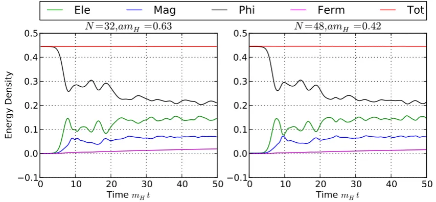
The lattice spacing dependence is shown in Fig. 4, showing the different energy

compo-nents on two different lattices with the same physical volume, but different lattice spacing

(N = 32, amH = 0.63 and N = 48, amH = 0.42). We see that by choosing the

0

5

10

15

20

25

30

Time

m

t

4

3

2

1

0

1

2

N

=4800

0

5

10

15

20

25

30

Time

m

t

4

3

2

1

0

1

2

N

=9600

Higgs

N

N

N

=(B+L)/2

Figure 2: The convergence of the baryon (or fermion) number requires much largerNq.

0

10

20

30

40

50

Time

m

t

0.1

0.0

0.1

0.2

0.3

0.4

0.5

Energy Density

0

10

20

30

40

50

Time

m

t

0.1

0.0

0.1

0.2

0.3

0.4

0.5

Ele

Mag

Phi

Ferm

Tot

Figure 3: Different energy component in a tachyonic electroweak transition. The Wilson

coefficient rw is 0 in the left plot, and 0.5 in the right plot. The energy density is scaled

by m4_H. More energy is transferred to the fermion when the Wilson term is small.

number of modes present), and so the agreement is quite non-trivial.

5 Spectrum

0

10

20

30

40

50

Time

m

t

0.1

0.0

0.1

0.2

0.3

0.4

0.5

Energy Density

N

=32

,am

=0

.

63

0

10

20

30

40

50

Time

m

t

0.1

0.0

0.1

0.2

0.3

0.4

0.5

N

=48

,am

=0

.

42

Ele

Mag

Phi

Ferm

Tot

Figure 4: The energy components in simulations at different lattice spacing but the same physical volume. Cut-off effects are well under control through tuning the counterterms accordingly.

Fermi-Dirac distribution will give the (effective) temperature and chemical potential of the system.

We define the correlation function in momentum space through a Wigner transform and averaging over the space volume,

D(p, t) = 1 V

Z

d3X

Z

d3ze−ip.zD(X+1

2z, X−

1

2z;t), (5.1)

which is equivalent to computing h|Tψ(p, t) ¯ψ(p, t)|i. For future use, we define:

F(p, t) = Tr[D(p, t)], V(p, t) = Tr[iγ.p

p D(p, t)]. (5.2)

A gauge-invariant correlation function for the gauge doublet can be defined as

DΨ(x, y;t) =h0|TΨ(x, t) ¯Ψ(y, t)U(y, x;t)|0i, (5.3)

where U(y, x;t) is the gauge link connecting x and y at the time t. For the gauge singlet

field, this is not needed

Dξ,χ(x, y;t) =h0|Tξ(x, t) ¯ξ(y, t)|0i, h0|Tχ(x, t) ¯χ(y, t)|0i. (5.4)

0

10

20

30

40

50

60

m

t

0.0

0.5

1.0

1.5

Higgs

0.0

0.5

1.0

1.5

2.0

2.5

3.0

3.5

aω

0.0

0.2

0.4

0.6

0.8

1.0

N

+

N

2

(

N

+

N

)

/

2

log

linear fit

0

2

4

6

8

10

lo

g(

2

N

+N

−

1)

Figure 5: The fermion particle spectrum (bottom panel). The red line is the average

particle number, the blue line the derived log(1/Nav−1), so that the slope is the inverse

temperature. The black line is the linear fit of the lower energy range. For the linear

fitting, we select the range aω ∈ [0,0.9]. The upper plot shows the time evolution of the

Higgs field observable and the time (mHt = 60.795) at which the spectrum is computed.

N = 48, amH = 0.63 andλyuk = 0.03.

weak eigenmodes (where the singlet correlator is gauge invariant) and the mass eigenstates for comparison.

The correlation function is expected to have the form [13]

D(p, t) = [1−N(p, t)−N¯(−p, t)]m(p, t)−ip.γ

2ω(p, t) + [ ¯N(−p, t)−N(p, t)]

iγ0

2 , (5.5)

which is obviously true for the setup (3.3) and (3.5). By assuming the on-shell condition

ω(p, t) =qp2_+m2_{(p, t), we have enough freedom to measure the effective energy ω(p, t)}

and the average particle numberNav(p, t)≡(N(p, t) + ¯N(−p, t))/2 simultaneously.

Nav(p, t) = 1

2 −sign[V(p, t)]

q

F2_{(p, t) +V}2_{(p, t)}

4 , (5.6)

ω(p, t) =

s

4(1−2Nav)2p2

0 10 20 30 40 50 60 70

Time

m

t

0

20

40

60

80

100

Temperature (GeV)

0 10 20 30 40 50 60 70

Time

m

t

200

150

100

50

0

50

Chemical Potential (GeV)

Unitary gauge fixing

Singlet

Doublet

Figure 6: Three definitions of the temperature and chemical potential. The red line is

extracted from the mass eigenstate (Ω1) after the unitary gauge fixing. The singlet and

doublet are extracted from the gauge singlet (ξ) and gauge doublet (Ψu) directly. N = 48,

Nq = 2400,λyuk=0.03 andamH = 0.63.

In the unitary gauge, the mass eigenstates Ω1,2 can be written in terms of the weak

eigen-states as

Ω1 =

1

√

2(Ψu+ξ), Ω2 =

1

√

2(Ψd+χ), (5.8)

Ω0₁ = √1

2(Ψu−ξ), Ω

0

2 =

1

√

2(Ψd−χ), (5.9)

where Ψu, Ψd are the up and down parts of the gauge doublet.

Having computed the particle number Nav(ω), we can proceed to extract the effective

temperature and chemical potential, by fitting to the form

log

1

Nav

−1

= ω−µ

T . (5.10)

If the system is properly equilibrated, the low-momentum range should indeed show this

form (Fig. 5).

To estimate the uncertainty from the gauge non-invariance, we have compared results

from different choices of correlators in Fig. 6 (left). The singlet (field ξ) is simply the

correlator (5.4) and doublet (field Ψu) is (5.3), but omitting the link variable. We compare

these to the temperature of an mass eigenstate (Ω1) in the unitary gauge (5.8). We see

that the doublet temperature deviates from the other two, with the unitary gauge one the smoothest. The right-hand plot shows the effective chemical potential, which only at later times becomes positive.

In Fig. 7 we show a comparison between difference ensemble sizes Nq demonstrating

0 5 10 15 20 25 30 35 40

Time

m

t

20

25

30

35

40

45

50

55

60

Temperature (GeV)

0 5 10 15 20 25 30 35 40

Time

m

t

100

80

60

40

20

0

20

40

Chemical Potential (GeV)

N

=9600

N

=2400

N

=1440

Figure 7: Convergence of the temperature and chemical potential with Nq. N = 32,

λyuk= 0.03 and amH = 0.42.

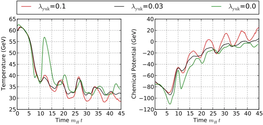
results for different values of the Yukawa coupling, Fig. 8. The valuesλyuk = 0.1, 0.03 and

0 correspond to fermion masses ∼ 17, 5.1, and 0 GeV respectively, and we see that the

temperature is largely independent of the choice of mass. This suggests that most of the energy transfer comes down through the gauge field coupling, rather than directly through the coupling to the Higgs. This conclusion may not hold for the top quark mass, which is high above the effective temperature. The dependence on the Wilson term coefficient was found to be comparable (not shown).

6 Fermion temperature in Cold Electroweak Baryogenesis

Cold Electroweak Baryogenesis assumes that the Universe came out of inflation around the electroweak scale, triggering a fast electroweak quench. The out-of-equilibrium dynamics of this tachyonic transition is then responsible for Baryogenesis, without a need for a first

order phase transition with bubble nucleation [9, 20–22]. It is known that the observed

asymmetry can be generated in the presence of a generic additional source of CP-violation

[10,11]. But extensive work has also gone into the possibility that the CP-violation already

present in the Standard Model through the complex phase in the CKM matrix may be

sufficient [2,19,23–25].

The status is that a number of effective bosonic operators arise upon integrating out the fermions at finite temperature, and the coefficient functions are strongly suppressed

with temperature. Bosonic simulations suggest, that the coefficient should be of order 10−6

in some normalization [11], corresponding to an effective temperature in the fermions of

0 5 10 15 20 25 30 35 40 45

Time

m

t

25

30

35

40

45

50

55

60

65

Temperature (GeV)

0 5 10 15 20 25 30 35 40 45

Time

m

t

120

100

80

60

40

20

0

20

40

Chemical Potential (GeV)

λ

=0.1

λ

=0.03

λ

=0.0

Figure 8: The effective temperature and chemical potential for different Yukawa couplings

λyuk= 0.1, 0.03 and 0, correspond to fermion masses ofmf = 17, 5 and 0 GeV respectively.

Nq = 2400,N = 32, andamH = 0.42.

30 20 10 0 10 20 30 40 50 60

Time

m

t

20

25

30

35

40

45

50

55

60

Temperature (GeV)

30 20 10 0 10 20 30 40 50 60

Time

m

t

100

80

60

40

20

0

20

Chemical Potential (GeV)

Figure 9: The effective temperature and chemical potential for a τQ = 30/mH quench.

Green bands denote statistical errors (1σ), over 8 bosonic realisations.

currently available. With the techniques outlined above, we are now in a situation to compute this effective temperature.

It is also known that generating the asymmetry requires the quench transition to be

fairly fast [12]. This is in order for the dynamics to be violent enough that non-perturbative

We now introduce a quench time as in [12] to parametrize the flip of the mass param-eters in the Higgs potential

V(φ) =µ2_eff(t)φ†φ+λ(φ†φ)2, (6.1)

with

µ2_eff(t) = µ2

1− 2t

τQ

, t < τQ, (6.2)

= −µ2, t > τQ. (6.3)

We then simulate the transition for different values ofτQ, in each case computing the

effec-tive temperature averaged during the first and second period of the Higgs field oscillation.

We use Nq = 2400, N = 48, lyuk = 0.03, amH = 0.63 and we in addition average over 8

realizations of the bosonic fields. An example of such an averaged effective temperatures

and chemical potential is shown in Fig. 9, at a quench time ofmHτQ= 30.

0

5

10

15

20

25

30

35

Quench time

(

)

22

24

26

28

30

32

34

36

38

Temperature (GeV)

1st Higgs minimum

2nd Higgs minimum

the late time limit

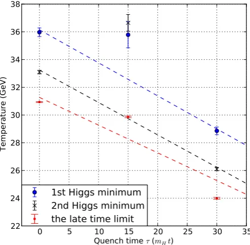
Figure 10: The first and second Higgs minimum correspond to the first and second time the Higgs field rolling back to the minumum of the average Higgs field squared. Each point

is the statistical result of 8 runs, with the error bar stands for σ confidential interval. The

statistical error for the late time limit is smaller than 0.2 GeV.

We finally show the effective temperatures at the first and second minimum of the Higgs

field, as well as the late time limit, as a function of quench time (Fig. 10). The effective

and it also decreases with quench time. For each of the measurement times (first, second minimum, late time), we can fit the temperature by a straight line. extrapolating these

to large quench times, we find that the required 1 GeV may be reached for mHτQ '150.

This is an order of magnitude slower than the requirements for a violent out-of-equilibrium

phase during the transition [12]. We conclude that Standard Model CP-violation cannot

be strong enough to generate the observed baryon asymmetry, also not in the context of Cold Electroweak Baryogenesis.

7 Conclusion

In summary, we have carefully developed the real-time lattice implementation of the

elec-troweak sector of the (reduced) Standard Model introduced in [1]. It includes the SU(2)

gauge and Higgs fields, treated classically, and one generation of fermions, treated quantum mechanically, using the ensemble fermion method. All the fermions are taken to have the same mass, around 5 GeV.

We found that the ensemble method converges for or order 2000 realisations of the fermions, for the dynamics and all observables except the fermion/baryon number. This is a reduction of the numerical effort by an order of magnitude, compared to what was

anticipated in [1], making the method viable for modelling the entire electroweak sector.

Including the full fermion spectrum, in particular the massive top quark will make

conve-gence slower. Our largest lattices (483, Nq= 2400) fill 135GB memory, which is certainly

tractable by modern supercomputers. Triple this for the full SM fermion content.

As an application of the method, we considered the tachyonic preheating mechanism after hybrid inflation, in the context of Cold Electroweak Baryogenesis. Standard Model CP-violation gives rise to effective higher order bosonic interactions, the coefficients of which are strongly temperature dependent. In order for SM CP-violation to be sufficient for generating the observed baryon asymmetry, we need a transient stage during preheating, where the fermions have a temperature in the region of 1 GeV. We find that the transient effective temperature in the IR is 10 to 20 times higher than this, lower for slower quenches. Extrapolation to very slow quenches potentially leads to a lower preheating temperature, but we come in conflict with the need for a far-from-equilibrium state also needed for successful baryogenesis.

We conclude that SM CP-violation is insufficient for baryogenesis, also in the Cold scenario. One caveat is that we have not included the top quark; however, since the top mass is about 5 times the largest temperature encountered here, only non-perturbative processes during the initial rolling down of the Higgs field can source it. We believe that this effect is unlikely to bridge the gap in temperature. Similarly, the reheating temperature

scales with the number of relativistic degrees of freedom as (g∗)−1/4, and so including all

the SM degrees of freedom (a factor of about 4 larger compared to what we have here, depending on whether W and Z are taken to be relativistic) also does not reconcile the measured temperature with 1 GeV.

wave creation during the electroweak phase transition, preheating dynamics in extensions of the SM as well as high temperature baryogenesis mechanisms where bubble walls sweep through a hot plasma. A first step is the implementation of the full three generations of the SM, with physical masses and mixings, and extensions of the Higgs sector, projects presently under way

Acknowledgments: The numerical simulations were implemented and performed on the COSMOS supercomputer, part of the DiRAC HPC Facility which is funded by STFC and BIS. ZGM wishes to thank Shuang-Yong Zhou and Paul Tognarelli for useful discussions.

A Fermion doublers and the Wilson term

In our simulation, we include only the spatial Wilson term to reduce the effect of fermion doublers,

SW =

Z

d4x rwa

2

_¯

ΨDiDiΨ + ¯χDi∂iχ+ ¯ξDi∂iξ

. (A.1)

The temporal doubler is suppressed by choosing the initial condition carefully, so that the doubler starts out un-excited. For a long enough simulation, the doubler mode will return, but we find that this happens on a timescale much longer than the simulations presented here.

Considering a single mode of theU part (withU one of the eigenspinors), which follows

the difference equation

γµ∆˜µUk(t) +mkUk(t) = 0, (A.2)

where the t is discretized into integer values, and on the first step Uk(1) =Ukeik.x. The

eigenspinor Uk is the solution of

−iγ0sink0Uk+iγisinkiUk+mkUk= 0, (A.3)

where the dispersion relation reads sin2k0 = P

isin2ki +m2_k. So here the recurrence

relation is

Uk(t+ 1)−Uk(t−1) =−i2 sink0Uk(t). (A.4)

The general solution is

Uk(t+ 1) =

e−ik0t

2 cosk0

[Uk(1)eik0 +Uk(2)] + (−)t

eik0t

2 cosk0

[Uk(1)e−ik0 −Uk(2)]. (A.5)

The second term on the right-hand side is the doubler and will switch the sign from step

to step. To remove it, one needs to select the initial condition that Uk(2) = e−ik0Uk(1),

and similarly,Vk(2) =eik0Vk(1) for theV part.

doubler parts by measuring three closest time steps,

ψp(x, t) =

ψ(x, t+ 1) + 2ψ(t) +ψ(x, t−1)

4 , (A.6)

ψd(x, t) =

ψ(x, t+ 1)−2ψ(t) +ψ(x, t−1)

4 . (A.7)

If there are only physical modes,

1

2hψ

†

pG(x, t)ψpG(x, t)ie = 1,

1

2hψ

†

dG(x, t)ψdG(x, t)ie= 0, (A.8)

and on the contrary, with only doubling modes,

1

2hψ

†

pG(x, t)ψpG(x, t)ie = 0,

1

2hψ

†

dG(x, t)ψdG(x, t)ie= 1. (A.9)

In practical simulations,A.8 is accurate up to the order of 10−5.

B Two-point functions on the lattice

For the Dirac field, the free two-point function has the form:

G0(x, y) =

Z π

−π

d4_p

(2π)4e

ip(x−y)_{G0(p) =}

Z π

−π

d4_p

(2π)4

eip(x−y) iγµ_sinp

µ+mp

. (B.1)

The wave number p is continuous if the size of the lattice N is infinite. For finite N, the

integral should be substituted by a sum overp= (2i−N+ 1)π/2, wherei= 0,1, ...N−1.

For any case,p is periodic with period 2π.

The above integral with the Minkowski signature contains on-shell poles for the real-time simulation. Different choices of open contour integration gives the definition of Feyn-man, advanced or retarded Green functions, and closed contour integrals will give the density function and statistical propagator.

The full two-point function can be expanded perturbatively if the interaction of the fermion and the background is weak. For the Higgs field background, if we choose the unitary gauge fixing and only consider zero component, the expansion is,

G(x, y) = G0(x, y)−λyuk

Z π

−π

d4k

(2π)4e

ikx_φ0(k)

Z

d4p

(2π)4e

ip(x−y)_{G0(p+k)G0(p), (B.2)}

up to the first order ofλyukφ0.

For the gauge field background, the perturbation is

G(x, y) = G0(x, y) +i

X

µ

Z π

−π

d4p

(2π)4

d4k

(2π)4Aµ(k)e

ikx_eip(x−y)_G

0(p+k)Γµ(p+k, p)G0(p)

+... (B.3)

where we have interpreted the gauge link as [Uµ(x)−1] =−iAµ(x), [Uµ†(x)−1] =iAµ(x)

to the first order. So the interaction vertex induced on the lattice is,

Γµ(p+k, p) = γ

µ

2 [e

−i(pµ+kµ)_+eipµ_{] +}rw

2 [e

The above perturbation respects the gauge symmetry, in the sense that the Ward identity is fulfilled in the form

iX

µ

(1−eikµ_)Γµ_{(p+k, p) =−iG}−1

0 (p+k) +iG

−1

0 (p). (B.5)

C Counterterms

We introduce counterterms for the back reaction of the quantum fermions onto the classical

bosonic fields. The full actionSC is chosen to be,

SC =−

Z

d4x

(Z3−1)

4 W

a

µνWa,µν+ (Zφ−1)Dµφ†Dµφ+δV(φ)

, (C.1)

The first term describes the screening effect when Z3 < 1, and will reduce the coupling

constant. In the equation of the motion for the Higgs field, the cancellation is

(Zφ−1)∂µ∂µφ0−

1

2δV

0

(φ0) = λyuk

Ψuχ+χΨu+ Ψdξ+ξΨd

2

= iλyukTr[G(x, x)−G0(x, x)], (C.2)

where G(x, y) and G0(x, y) are Green functions for different mass eigenstates in the weak

theory. For the gauge field

4(Z3−1)

g2 (E

a

n(x)−Ena(x−0)−

4(Z3−1)

g2

X

m

Dab_m0TrhiσbUx,mUx+m,nU

†

x+n,mUx,n†

i

= hΨ¯xγniσaUx,nΨx+n+ ¯Ψx+nγnUx,n† iσaΨx

i −rw

h

¯

ΨxiσaUx,nΨx+n−Ψ¯x+nUx,n† iσaΨx

i

= iTr[iσaUn(x)G(x+n, x)γn] +iTr[Un†(x)iσaG(x, x+n)γn]−irwTr[iσaUn(x)G(x+n, x)]

+irwTr[Un†(x)iσaG(x, x+n)]. (C.3)

Using the perturbative Green functionB.2andB.3, the coefficients of the counterterms can

be computed. We perform the contour integral in continuous energy first. For instance,

Z π

−π

dω

2π

B

sin2ω−sin2c+i =−2i

B

sin 2c, c∈[0,

π

2]. (C.4)

This leaves three dimensional discretised lattice sums, which are computed numerically. We choose the counterterm for the potential

δV = ct1

2 φ

2₊ct2

4 φ

4_{, (C.5)}

where ct1 depends on the lattice spacing quadratically, and ct2 depends on the logarithm

of the lattice spacing. φ can be set to be constant in B.2 and C.2 to get the ct1 and ct2

quickly. To obtain Z3 and Zφ, one may select the field to have a particular momentum

to simplify the calculation. With our choice of lattice parameters, 0.98< Z3 <0.99, and

References

[1] P. M. Saffin and A. Tranberg, JHEP1202(2012) 102 [arXiv:1111.7136 [hep-ph]].

[2] T. Brauner, O. Taanila, A. Tranberg and A. Vuorinen, Phys. Rev. Lett.108(2012) 041601 [arXiv:1110.6818 [hep-ph]].

[3] M. D’Onofrio, K. Rummukainen and A. Tranberg, JHEP1208 (2012) 123 [arXiv:1207.0685 [hep-ph]].

[4] K. Kajantie, M. Laine, K. Rummukainen and M. E. Shaposhnikov, Phys. Rev. Lett.77(1996) 2887 [hep-ph/9605288].

[5] E. J. Copeland, S. Pascoli and A. Rajantie, Phys. Rev. D65(2002) 103517 [hep-ph/0202031].

[6] A. Rajantie, P. M. Saffin and E. J. Copeland, Phys. Rev. D63 (2001) 123512 [hep-ph/0012097].

[7] J. Garcia-Bellido, M. Garcia-Perez and A. Gonzalez-Arroyo, Phys. Rev. D69(2004) 023504 [hep-ph/0304285].

[8] A. Diaz-Gil, J. Garcia-Bellido, M. Garcia Perez and A. Gonzalez-Arroyo, Phys. Rev. Lett. 100(2008) 241301 [arXiv:0712.4263 [hep-ph]].

[9] A. Tranberg and J. Smit, JHEP0311 (2003) 016 [hep-ph/0310342].

[10] A. Tranberg and J. Smit, JHEP0608(2006) 012 [hep-ph/0604263].

[11] A. Tranberg, A. Hernandez, T. Konstandin and M. G. Schmidt, Phys. Lett. B690(2010) 207 [arXiv:0909.4199 [hep-ph]].

[12] A. Tranberg, J. Smit and M. Hindmarsh, JHEP0701(2007) 034 [hep-ph/0610096].

[13] G. Aarts and J. Smit, Phys. Rev. D61(2000) 025002 [hep-ph/9906538].

[14] G. Aarts and J. Smit, Nucl. Phys. B555(1999) 355 [hep-ph/9812413].

[15] S. Borsanyi and M. Hindmarsh, Phys. Rev. D79(2009) 065010 [arXiv:0809.4711 [hep-ph]].

[16] F. Hebenstreit, Jr. Berges and D. Gelfand, Phys. Rev. D87(2013) 105006 [arXiv:1302.5537 [hep-ph]].

[17] F. Hebenstreit, Jr. Berges and D. Gelfand, arXiv:1307.4619 [hep-ph].

[18] P. M. Saffin and A. Tranberg, JHEP1107(2011) 066 [arXiv:1105.5546 [hep-ph]].

[19] T. Brauner, O. Taanila, A. Tranberg and A. Vuorinen, JHEP1211 (2012) 076 [arXiv:1208.5609 [hep-ph]].

[20] J. Garcia-Bellido, D. Y. Grigoriev, A. Kusenko and M. E. Shaposhnikov, Phys. Rev. D60 (1999) 123504 [hep-ph/9902449].

[21] L. M. Krauss and M. Trodden, Phys. Rev. Lett.83(1999) 1502 [hep-ph/9902420].

[22] E. J. Copeland, D. Lyth, A. Rajantie and M. Trodden, Phys. Rev. D64(2001) 043506 [hep-ph/0103231].

[23] A. Hernandez, T. Konstandin and M. G. Schmidt, Nucl. Phys. B812(2009) 290 [arXiv:0810.4092 [hep-ph]].

[24] C. Garcia-Recio and L. L. Salcedo, JHEP0907(2009) 015 [arXiv:0903.5494 [hep-ph]].